How to Compute Earned Hours and Direct Headcount for Standard Costing

Cost Accounting 101 – Earned Hours and Direct Headcount

To compute earned hours and direct labor for standard costing plan requires you to first determine how many hours of labor are going to be required given your build plan.  This is why we are frequently asked how to compute earned hours and direct headcount, which we have been doing for many years.  This is one of a four-part series on manufacturing cost accounting.  After you have had a chance to better understand how to compute earned hours and direct headcount, take a look at the following to enhance your knowledge:

How to Compute Overheads Rates and Utilize Variances

How to Create a Profit and Loss Statement for a Manufacturing Business

How to Compute Direct Labor Rates

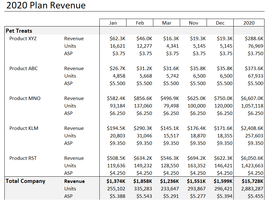
Developing the build plan requires input from both Marketing/Sales to identify what is going be shipped, in what quantities and in what month.  Here is an example of a typical revenue plan that could be generated by Marketing/Sales:

In this example, the important lines are the Units sold or shipped.  To simplify the example, we are going to produce the units sold in the month the units are to be sold without giving consideration to inventory levels, safety stock, service levels, etc.  But in a more realistic situation, all those factors would be combined with the units shipped below to compute a demand plan that more closely aligns with organizational goals for total inventory.

How to develop a build plan

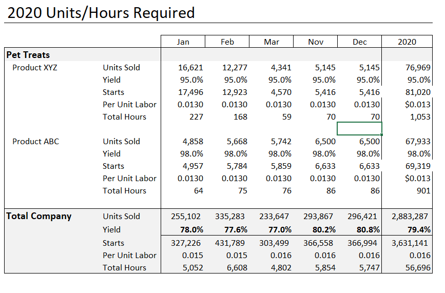
Using the revenue plan as the starting point for our build plan, the next step is to factor in a yield rate.  Looking at our example below, you can see that Product XYZ has a planned yield rate of 95%, which means that we plan to scrap 5%.  There are some nuances to consider relative to how you factor in scrap, but for now we are just increasing the units needed by the yield (Units Finished / Yield %), to compute the units started.  Again, looking at the month of January for Product XYZ, we need to finish 16,621 to ship that same quantity.  To have 16,621 complete, we need to start 17,496 units when the expectation is to scrap 5% of the units started.  

Manufacturing Engineering provided the per unit labor standard for Product XYZ, which was set at .0130 hours per unit, which when multiplied by the number of starts–17,496–indicating a need for 227 hours of direct labor build time to complete this requirement.  We go through the same process for all 5 products for the entire year.  Though many rows and columns are hidden on the image below, you can see the totals for all the products at the bottom of the worksheet.  You can review the results below and see that the total number of hours of direct labor required to finish 2,883,287 units is 56,696 hours.  The 56,696 hours flows into our headcount plan model. 

As we mentioned there are some consideration you need to make regarding how to plan for scrap.  One of the first considerations is how does your ERP system handle scrapped units.  Do you scrap units off the work order before any direct labor is earned?  Or do you scrap units after the work order is confirmed, which includes the earned hours in the scrapped unit.  This has implications for both how you plan scrap and overhead absorption.  So be sure you understand where the confirmation process for each good and bad unit occurs to more accurately estimate production variances.  Our hypothetical ERP system is assumed to scrap units after confirmation, which increases the cost of scrap and decreases potential labor efficiency variances.

Final Step — Converting earned hours into direct labor headcount.

Our final step in how to build an earned hours and direct labor plan uses many of the same assumptions that were used to compute our direct labor rate in our post on How to Compute a Direct Labor Rate.  If you did not read that post, you may want to take a minute to review it so you will better understand some of the assumptions being used here. 

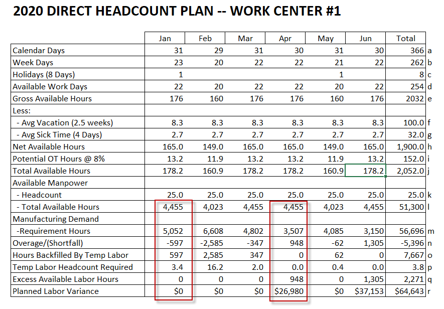
The final result is below, with several of the months hidden to accommodate our screen width.  Below we describe each row in more detail, but essentially the point of this exercise is to see where you may potentially have too much headcount or too little headcount.  If you reviewed our post on How to Compute a Direct Labor rate, you may recall that our rate calculation assume 25 full time employees, which has carrier over to this example, along with all the same assumptions regarding holidays, vacation time, sick pay, etc.  Please review the summary below and continue on for a deeper explanation on all the calculations to understand how direct headcount required is computed:

Here is an explanation of the various rows, using the letters in the right margin:

1. Calendar Days is just the days in each month.  Note that 2020 is a leap year, bringing the total number of days to 366.
2. Work Days is just that, the number of work days in a given month.  You would guess that the number should be 260 days (5 days a week * 52 weeks), but it is actually 262.  There is one extra day and the extra day for leap year brings the total to 262.
3. Holidays are spread out to the months when they will occur.  There are 8 holidays provided by our hypothetical company.
4. Available work days is the total work days at b) less the holidays (262 work days – 8 holidays = 254 available work days.
5. Gross available hours is computed by multiplying 8 hours (our hypothetical company has a nominal 8 hour work day) by the available work days at d).
6. Now we subtract the potential vacation hours we expect the average employee to take, which is just straight lined for the year.  The assumption is 2.5 weeks or 100 hours for the year.  We suggest using historical vacation utilization reports to make this a bit more accurate, but this is just an example.
7. We also want to subtract from gross available hours our expectation for Sick hours, which was 4 days or 32 hours for the year.  Again this is just straight lined across the year, but could be refined if desired using historical payroll information.
8. Net Available hours is our Gross available hours less vacation (f) and sick time (g).  This is essentially the straight-time hours we expect the average employee to be on site and available for work, before accounting for any overtime, which is 1,900 hours per year.
9. We are just bringing over our overtime assumption from the direct labor rate calculation, which is an additional 8% of hours.
10. Total Available Hours is the total number of hours we expect employees to be producing value for the company.  In 2020, this was 2,052 hours per employee.
11. Available Headcount, as we mentioned earlier, is expected to be 25 full-time employees for this work center in 2020.
12. Available Hours is multiplying the monthly headcount by the monthly Total Available Hours at j.
13. The Requirement Hours are just coming from the yielded build plan that was based on the sales volume.
14. The Overage/(Shortfall) line is just the difference between the Available Hours at l minus the Requirement Hours at m.  A positive variance indicates that we have more manpower than is demanded in form of Requirement Hours.  Assuming that we were going to back fill the months with a Shortfall using contract labor, then the Overage hours would be unfavorable labor variance and should be part of the Variance Forecast.  If the plan is to modify the production timing to accommodate the total Requirement Hours, then no variance will be generated.  A Shortfall–more Requirement Hours than Available Hours–is assumed to be solved using contract labor, in which case there would be no efficiency variance.  Note: In our labor rate forecast we did not include an assumption for Contract Labor.  If you have this issue, you may want to revisit your Direct Labor Rate computation to adjust for adding in some amount of contract labor. 
15. Again, a Shortfall is assumed to be filled by Temporary Labor.  This row has the hours required to be back filled by Temporary Labor.  As you can see, the total hours of Temp Labor back fill is 7,667 hours, which translates into almost 4 man years of labor. 
16. Total Temp Headcount Required is just converting the monthly Shortfall hours at o, into headcount.
17. Both lines q and r are about computing the unfavorable labor variance, in hours and heads respectively, due to the surplus hours.
18. Labor Variance Dollars would be integrated in your P&L plan.

In an earlier post, we describe the process for computing the monthly labor variance, which is comprised of a rate component and an efficiency component.  We suggest you review the the How to Compute a Direct Labor Rate post for more details, then you will more fully understand and modify your approach to computing earned hours and direct labor for standard costing.

Hope fully you found this enlightening and can utilize it in your own organizations.  If you need help setting up your revenue and build plans, please give us call.  If you would like a copy of any of the workbooks used as examples, reach out.  We have the tools to help.