CONTENTS
-
- Looking under the hood requires getting into the detail, which entails getting your hands a little dirty
- So what is ROE?
- What is the DuPont Equation or Formula?
- Using the DuPont Formula to super charge a business
- A more analytical approach using Microsoft Excel Solver
- What would Donaldson Brown think today?
How to Use DuPont Analysis and ROE to to Super Charge your Business
Using DuPont Analysis requires getting into the detail, which entails getting your hands a little dirty
If you have ever watched a mechanic diagnosis problems on a modern car, you will have noted that the process begins with the mechanic plugging in an electronic scanner. The scanner enables the mechanic to quickly identify electronic and mechanical issues with your vehicle. This vastly reduces the amount of time the mechanic has to spend determining the root cause of your problem. Using ROE to analyze and improve business performance is analogous to a mechanic using a scanner to diagnosis what’s ailing your vehicle.
The actual tool used to analyze ROE is the the DuPont analysis (or formula), which is aptly named given that it was developed at the DuPont Corporation way back in the 1920s. The employee that created this methodology–Donaldson Brown–used the DuPont equation to evaluate, compare and improve DuPont’s far flung business operations. Of note, Brown later moved on to GM and worked with Alfred Sloan to super charge General Motors from 1936 through 1946, indirectly helping with America’s war effort. Though Brown used his equation on an expansive scale, the DuPont equation can provide valuable insight and keys to business performance improvement for entities both large and small; consequently, we are going to describe how to use ROE to go under the hood and super charge your business.
So what is ROE?
ROE is a measure of return or profitability from a shareholder’s or owner’s perspective, given that it is the result of dividing net profit by equity. Because equity represents stakeholders’ investment, ROE reflects the return shareholders are realizing on that investment. This facilitates a shareholders ability to compare an investment in business XYZ to other investment opportunities. But there are other reasons to focus on ROE, one of the primary reasons being that ROE equalizes many of the factors that affect businesses in completely different industries, e.g. businesses with low profit margins because of fierce competition or huge investment outlays due to long development cycles and distills all those factors into one meaningful metric–ROE.
This means that two companies with very different business models, because each company operates in a different industry, can get to the same ROE using different strategies. But there are other reasons to focus on ROE, one of the primary reasons being that ROE equalizes many of the factors that affect businesses in completely different industries, e.g. low profit margins because of fierce competition, huge investment outlays due to long development cycles, etc., and distills all those factors into one meaningful metric for comparison–ROE.
For example, J&J a large consumer products, medical device and pharmaceutical company can have a ROE that is very similar to Walmart, a large brick and mortar and internet retail company. Both have loads of inventory, but J&J has significant assets in accounts receivable, where Walmart has practically none. J&J generates has huge gross margins (≈65%), while Walmart is fairly thin (≈25%). So how do these disparate businesses get to relatively the same return, or ROE, for their shareholders? Read on to learn how…
What is DuPont Analysis or Formula?
The DuPont analysis will help us begin peeling away, or decomposing, the major factors affecting financial performance and provide a “drill down path,†using a little algebra. This is the getting your hands a little dirty part. So pull out your financials statements and let us begin…
Initially, we will us DuPont analysis to separate ROE into three components– profit margin, asset turnover (or asset utilization efficiency) and financial leverage. Later will will further decompose the factors affecting ROE.
Decomposing ROE into 3-part formula
First we begin with the basic ROE formula which is:
ROE = Net Profit / Equity
Next, we can decompose ROE into Return on Assets (Net profit / Assets) or ROA and financial leverage (Assets / Equity), as follows:
ROE = Net Profit / Assets * Assets / Equity
ROA measures a company’s return on their total assets. Again, depending on the industry, some companies have a higher ROA than companies in completely different industries. But companies in the same industry can produce the same ROE by utilizing financial leverage differently. The financial leverage, computed by dividing assets by equity, measures how shareholder money is being leveraged to deploy the assets required to generate sales. A financial leverage equal to 1.0 means essentially no leverage, since shareholders have provided every dollar used to deploy the required assets. A financial leverage of 3.00 indicates that for every dollar of assets, $0.33 has been provided by shareholders while the other $0.67 has been provided by vendors (in the form of AP) and banks (in the form debt). Financial leverage increases as shareholders own a smaller piece of total assets, which means our lenders have a greater claim on corporate assets.
Now we decompose the ROA part of our two-part formula into a three-part formula as follows:
ROE = Net Profit / Sales * Sales / Assets * Financial Leverage
Net profit divided by sales is Return on Sales (ROS), which we can think of as a measure of how effectively a company is able to recover their cost of goods sold after delivering whatever products and/or services they provide, as well as all other expenses. This is an important metric when comparing companies within an industry; consequently ROS is a good Industry benchmark, but it does not indicate how much money is going into the bank, which is what we really care about at the end of the day.
Sales divided by assets can be thought of as a turnover metric. Our turnover metric tells us how fast we are able to turn over assets in support of generating revenue. An asset turnover metric of 2.0 indicates that a business is able to turnover assets twice a year. Higher the turnover, the better because it reflects management’s ability to efficiently utilize assets. Think of assets are just piles of cash that need to be minimized in the pursuit of revenue.
Decomposing ROE into a 5-part formula
Now we can expand the three-part formula to a five-part formula that will help us analyze ROS in a little more depth. First we are going to remove the tax component from net profit by adjusting our ROS as follows:
ROS = Net Profit / Sales = Net Profit / Pretax Profit * Pretax Profit/Sales
Then finally, we are going remove the impact of interest expense, which is a reduction to operating margin, to isolate our operating margin or Earnings before Interest & Taxes (EBIT), as follows:
ROS = Net Profit / Sales = Net Profit / Pretax Profit * Pretax Profit / EBIT * EBIT / Sales
Replacing the ROS calculation in the three-part formula with the above, we now have a five-part formula for ROE, which is as follows:
ROE = Net Profit / Pretax Profit * Pretax Profit / EBIT * EBIT / Sales * Asset Turnover * Financial Leverage
Using the DuPont formula above, we can quickly compare companies and begin to see where there are differences in operating efficiency, asset utilization and leverage. With this information, we can then begin to drill down further. For example, if we note a significant difference in asset utilization, more than likely that difference is going to exist in accounts receivable and/or inventory. With detail in hand, we use both days sales receivables (DSR) and days inventory on hand (DIOH) to better understand the differences.
A ROE Example
Assume that we have been tasked with comparing Our Company to another rival in our industry (Company B). Both companies have similar ROEs, but Our Company has significantly higher revenue. So we start by lining up the basic financial statements for the two companies as referenced below (note that rather than comparing two companies, this same analysis could be used to compare the same company over time):
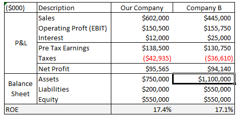
As we can see from above Company B generates less revenue, but delivers a very similar ROE. Since both companies are in the same industries and have the same equity, we need to determine where the differences exist. We start with the three-part formula, which produces the following result with comments on the results:
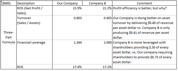
Now we can start to see some of the differences that are helping Company B’s performance. For starters, their ROS is 21.2% vs. Our Company’s 15.9%. It is not clear what the drivers are of better profitability, but we will get to that. Our Company has the better asset turnover ratio, generating $0.80 of revenue per asset dollar vs. Company B generating $0.41 of revenue per asset dollar. Finally, Company B uses financial leverage more aggressively than Our Company, only using $0.50 to fund a dollar of assets vs. Our Company is funding each asset dollar with $0.73 of equity, which is a significant part of the difference.
Now we will expand to the five-part formula to better understand the differences in ROS, which is below.
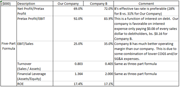
Now we can start to see some of the drivers for differences in ROS. First, the marginal tax rate for Our Company is a bit higher than Company B (28% for Company % vs. 31% for Our Company). Company B has a less favorable Pretax Profit to EBIT ratio because Company B services more debt (interest expenses). Finally, Company B has a much better operating margin which could be the result of a number of factors, but provides some hints regarding the difference (most likely this is going to be some combination of better gross margins and lower Operating Expenses).
Using the DuPont Formula to super charge a business
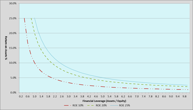
Assume that management would like to see the current ROE increased to 25%. We can use our DuPont analysis and some graphing skills to analyze the changes required to achieve a 25% ROE. First we start with a template where we plot the potential ROE outcomes for a 10% ROE line, 20% ROE line and 25% ROE line. We are only going to use the two-factor formula, which is as follows:
ROE = Net Profit / Assets * Assets / Equity or ROE = ROA * Financial Leverage
On the graph, we will use ROA for the Y axis and Financial Leverage for the X axis. In order to create our ROE lines, we start with the ROE 10% line and then determine what combinations of ROA and financial leverage will generate a 15% ROE. To plot the line, we solve for ROA (you can solve for either ROA or Financial Leverage), by dividing the desired ROE by each financial leverage interval we want to plot. So for example, at a 1.5 Financial Leverage (or interval), to plot a 10% ROE data point we just need to divide the 10% ROE by the 1.5 financial leverage to derive a 6.7% ROA. By doing the same for all the intervals of financial leverage for ROEs of 10%, 20% and 25%, we get the following:
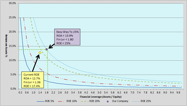
Next, we have graphed our current ROE performance as well as extrapolated the current performance diagonally to the 25% ROE goal and computed the ROA and financial leverage along the 25% ROE curve. We extrapolated out diagonally because this solution requires a measured improvement in both profitability and financial leverage. The new graph appears as follows on the next page:
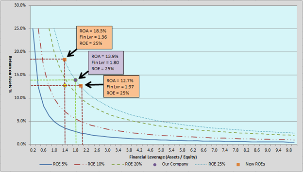
If desired, we can bound our solution by determining the upper and lower limits of our solution by determining what the ROA is required to produce a 25% ROE when holding the financial leverage constant at 1.36, as well as determining what financial leverage is required to produce a 25% ROE when holding ROA constant at 12.7%. These data points appear as follows:
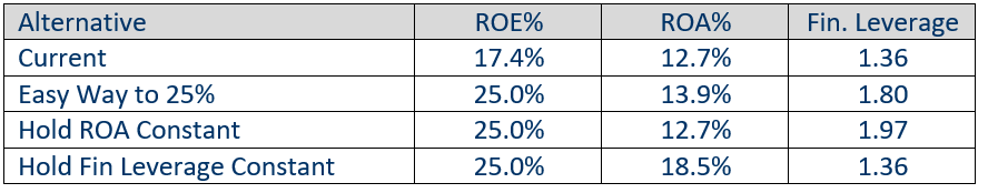
In the table below we have summarized a number of ways to go from our current ROE performance to achieve a 25%. We can now use this data to start to evaluate approaches to actually realize the 25% ROE by looking at gross profit, operating profit and net profit as it relates to total assets. The question for ROA performance is can we improve profitability without increasing assets proportionally or can we reduce assets while not decreasing profitability proportionally and the same goes for financial leverage. With this information, we can start to get further into the details adjusting days sales on receivables, inventory turns, days payables outstanding, as well our effective tax rate assumptions, to analyze our alternatives.
A more analytical approach using Microsoft Excel Solver to Perfect DuPont Analysis
Our Easy Way to 25% presented above, is conceptually easy but in reality probably infeasible. Certainly, increasing the ROA from 12.7% to 13.9% seems realistically achievable. Changing the Financial Leverage from 1.36 to 1.80 is huge. Remember that assets are in the numerator. Assuming that we are not going to be decreasing equity–the number in the denominator—we have to increase assets 32%+, with the offset most likely going to debt. This would certainly increase shareholder financial leverage, but seems a bit aggressive unless we have a good uses for all those assets.
Excel Solver is an add-in program that comes with all current versions of Excel. So you already have access to Solver, you just have to enable its use in Excel. We are now going to use Solver to help us optimize our ROA and Financial Leverage targets with a little more granularity than was used in the graphical solution. First we need to break out a few details from our summarized P&L and balance sheet that had been presented on a consolidated basis earlier in this article. Our company financials now appear as follows:
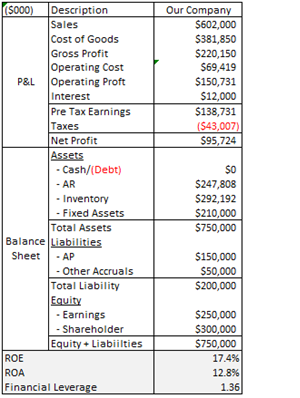
You can see that we essentially have all the same values as the earlier model, but have broken out cost of goods, operating expense, accounts receivable, inventory, fixed assets, accounts payable, other accruals, debt and our two equity components—earnings (or retained earnings) and shareholder equity.
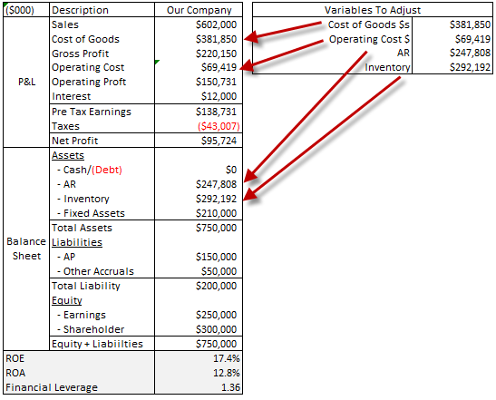
We are going to want Solver to alter certain aspects of the above financials to achieve our 25% ROE target. We can change just about anything using Solver, but for now we are going to keep it simple. So what we are going to want Solver to adjust the following items: 1) cost of goods sold, which will affect our gross margin; 2) operating expenses, which will affect our operating margin; 3) accounts receivable, which will affect total assets and be discernible through changes to our Days Sales of Receivable Outstanding or DSO (This is basically a measure of the number of days of sales represented by the current balance in accounts receivable. For example, if we $100K in sales in the current month, and we have $100K of receivables, then one could say that we have 30 days of sales in receivables or DSO = 30 days.); and 4) inventory, which will affect total assets as well and be discernible through changes to Days Inventory On Hand (This is similar to DSO, but is based on the average daily cost of goods. This means that if we have $200K of inventory and we incurred $50 in cost of goods during the most recent month, we would conclude that there are 120 days of inventory on hand ($200K Inventory / $50K cost of goods in current month * 30 days = 120 DIOH.).
We now need to adjust our model to consolidate the values Solver will vary when seeking our target goal. To accomplish this, we created an area on the worksheet that summarizes the four values to be altered and then link them back to the financial statements as shown below:
The next step is to establish the constraints that Solver will use to find a feasible solution to get us to 25% ROE. We are going to add the following constraints to our model so that we do not end up with another infeasible 25% ROE solution similar to the graphical solution. For the first iteration of the Solver model will utilize the following constraints:
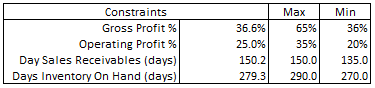
As can be seen, we are going to add four constraints, which include Gross Margin and Operating Margin target ranges. The DSO and DIOH metrics will guide Solver to produce solutions that reflect some level of asset efficiency improvement off of current results, which are 150 Days Sales Receivable (DSR) and 279 Days Inventory On Hand (DIOH).
With our baseline model set up and constraints defined, we need to get all this information loaded into Solver. Solver is available on nearly all Excel installations, but Solver needs to be selected as an available Add-in. In Excel 2016, this is done using the File tab, Options, and Add-ins screen, which generated the following dialog box on the next page:
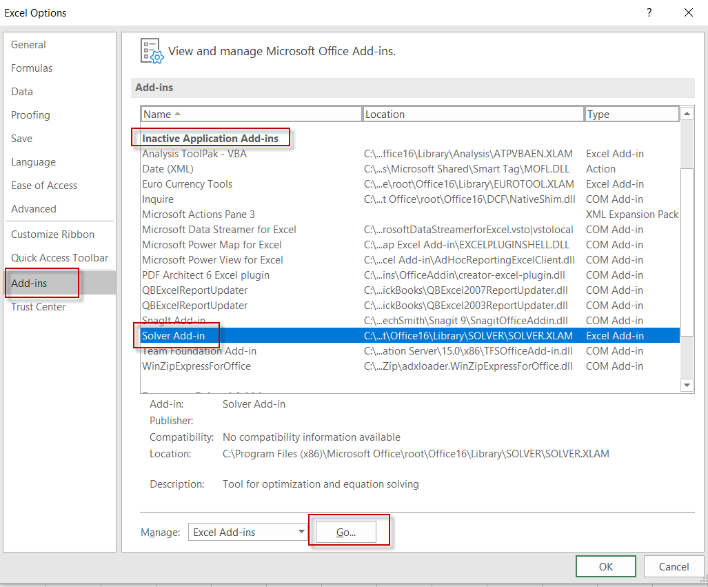
Note that in the above example, Solver Add-In is beneath the Inactive Application Add-Ins category. We select Go… which brings up a dialog that allows us to check the Solver application, which will then move the Add-In into the Active Application Add-Ins category.
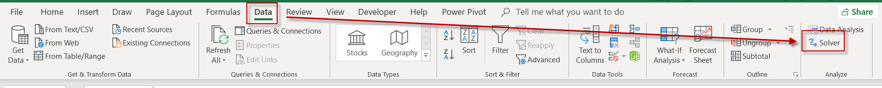
In Excel 2016 (it will available in a different location if you are using an earlier version of Excel), Solver is available on the Data Tab, in the Analysis group as shown below:
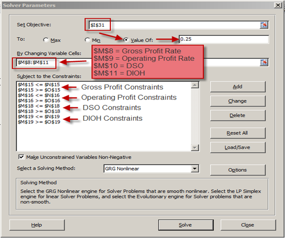
We just click on the Solver menu option to begin defining our model. The first step is to define the goal (25% ROE) and the location of the ROE calculation (cell I31 in our example spreadsheet). Next we need to identify the location of the four values to be varied–gross profit, operating profit, DSO, and DIOH (cells M8:M11). The last step is to create the constraints. Using the add buttons, we added constraints for gross profit, operating profit, DSO and DIOH. The buttons to the right of the constraint dialog were used to add the eight constraints (a <= and >= for each constraint). The completed Solver dialog for our initial model appears as follows on the next page:
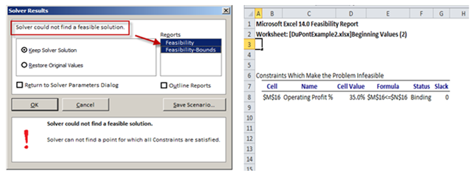
With our target set, variable cells identified and constraints established we select the Solve button to run our initial model. After our initial run, Solver responds back that it could not find a feasible solution given our constraints. If we check the “Reports†option, we get additional information on which constraint(s) is preventing Solver from finding a solution. Below, we have captured both the Solver Result indicating that there was no feasible solution as well as the feasibility report identifying our Operating Profit constraint (maximum of 35%) as the variable that needs to be adjusted before Solver can find a solution.
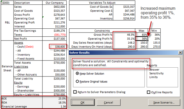
With this information, we now increase the Operating Profit maximum slightly from 35% to 36% and rerun the Solver model. To change the maximum on the constraint, we just need to update the values on the constraint table. After increasing Operating Profit percentage and rerunning the model, Solver was able to find a feasible solution, which appeared as follows:
Findings from Solver Results
The DuPont model factors are summarized at the bottom left of the graphic above and shows us achieving our targeted 25% ROE with an ROA of 18.3% and an unchanged financial leverage. Note that we are not changing liabilities, nor equity; consequently assets are going to remain at $750K. We could build a model to vary liabilities and equity, but for now we are keeping the model fairly simple. Given that assets are going to remain the same, the financial leverage is going to remain constant. But the focus in this model should be on what happens to cash. In the beginning model, we set cash to $0. As we push for more aggressive accounts receivable and inventory assumptions, then cash will increase to maintain assets at $750K.
As you will recall from our graphical solution, we just duplicated our graphical solution that held financial leverage constant and adjusted ROA to achieve ROE of 25%. But with this model, we have much greater insight into what is required to achieve this goal, such as how much surplus cash can be created by gaining more efficiency in DSR and DIOH, as well as where the constraints exist in our assumptions. With some time and effort this model could be modified to allow adjusting liabilities, if desired. With more time and experimentation with similar models, you can make more realistic models that accurately reflect a given situation that identifies various strategies for super charging your business!
What would Donaldson Brown think today?
I am guessing that Mr. Brown would be overjoyed with the ease with which he could deploy his DuPont formula to optimize financial performance for both DuPont and GM. Hopefully this blog post inspires you to take action and use ROE to go under the hood and super charge your business.
If you are a business owner that is looking for ways to leverage financial planning, cost accounting and/or data analytics to improve and grow your business, please contact us today.