CONTENTS
-
- Why Should You Analyze Gross Margin Variances
- Step #1 – Compute Average Sales Price Variance
- Step #2 – Compute Average Cost Variance
- Step #3 – Compute Sales Volume Variance
- Step #4 – Compute Cost Volume Variance
- Step #5 – Compute Family-Level Volume Variance
- Step #6 – Compute Family-Level Mix Variance
- Step #7 – Review the Gross Profit Bridge Variances
- Step #8 – Review Gross Margin Bridge Variances
- Step #9 – Get Copy of Gross Profit/Margin Template
9 Steps to Generate an Insightful Gross Margin Bridge Using Excel
This guide is designed for financial planning & analysis professionals, cost accountants and other analytical staff at midsize businesses who want to master gross margin analysis to drive better business decisions. A critical part of analyzing profitability is being able to bridge your planned vs. actual gross profit variance when reviewing monthly and year-to-date results, as well as vs. prior year. Analyzing sales variances is fairly easy, because it just falls to just price (or ASP) and volume variances. If you would like to learn how to build a gross profit plan, which requires a revenue and cost of goods plan to compute gross profit, see our How to Build a Time-Phased Sales and Cost Plan for Gross Margin Analysis blog post. But gross margin analysis is a little more complex given that it includes both cost and mix variances in addition to price and volume components. But don’t fret because we are going to take you through a detailed analysis looking at all four. Before we begin peeling away various aspects of gross margin variance, let’s define where gross margin comes from. Gross margin starts with under standing the gross profit formula, which is as follows:
Gross Profit = Price – Cost of Goods
Price is typically the amount invoiced a customer for a given product or item and is normally reflected on an invoice to a customer. Cost of Goods is the cost incurred by a business to either manufacture or procure the item sold. For a manufacturer, Cost of Goods will include the cost of direct materials, inbound shipping, direct labor, overhead, scrap, etc. For a distributor, Cost of Goods will include the cost of the items purchased for sale, along with some added overhead burden and inbound shipping cost to produce a fully landed cost of goods. In either case, you can think of Cost of Goods as both the variable and fixed cost costs required to transform a set of inputs into some tangible item that can be sold for more than the total cost inputs to an end customer (hopefully). Gross Margin is computed as follows:
Gross Margin Percentage Formula = Gross Profit / Price
Gross Margin is the percentage of Price that is greater than the cost inputs used to transform a set of cost inputs into something a customer is willing to purchase. The greater the gross margin, the more customers are willing to pay above the total cost inputs. Without this positive differential, there is no viable business model; consequently, being able to analyze gross margin as compared to both a plan and prior years, as well taking action on those insights, is an existential imperative for any product-based business.
What insight can be gained from a gross profit/margin analysis?
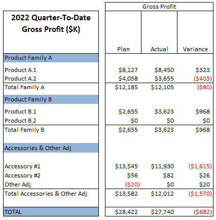
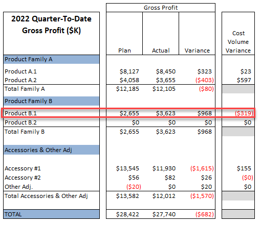
Referenced below is a typical plan vs. actual comparison, for a quarter-to-date time period, that solely provides the raw Gross Profit variances (remember, this is Price less Cost equals the results below). The report is summarized by Product Groups that are summarized into Product Families. You can use whatever terminology you prefer regarding the summary, but depending on the size of the business, a product hierarchy will facilitate forecasting and analysis of various product lines, families, types or whatever terminology your organization uses to segment business results. The result below, which could just as easily be comparing this gross profit to last, provides the total gross profit variance, but is just a starting point on our quest to develop some actionable insight:
After viewing a summary like the one above, and being the inquisitive type, you are going to want to drill down into the source of the $682K unfavorable variance. Here are some common questions you might ask:
- Is our pricing strategy working as planned?
- What is the gross profit impact of new products?
- How are volume differences within a product family or group impacting gross profit?
- Are our assumptions regarding standard/average costs (or prices for that matter) correct?
- Are volume vs. price vs. mix favorably, or unfavorably, impacting total gross profit and if so, by how much?
- Which products/families/types are having the greatest impact to gross profit, both good and bad?
- Given our options for influencing gross profit, what will have the greatest “bang for the buck?”
Step #1 – Determine what part of the total variance can be attributed to Average Sales Price (ASP) differences
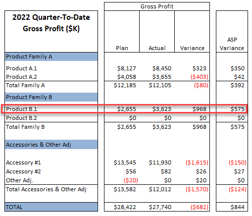
As an example, we will drill into the Product B.1 variance, starting with the ASP Variance impact. ASP is computed by dividing gross invoice price by the number of units shipped. An ASP Variance is computed as follows:
ASP Variance = (ASP Actual – ASP Plan) * Actual Volume (or units actually shipped)
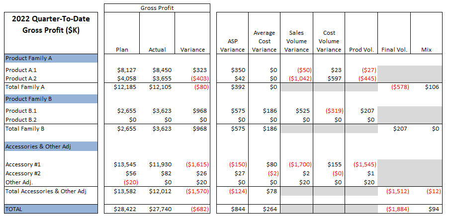
Below are the ASP Variances for all the Products. We will spend time drilling into the Product B.1 variances, which totals $968K favorable, with $575K associated with the ASP Variance.
Viewing the 1Q plan vs. actuals for Product B.1 on our supporting schedules (shown later), the plan assumed that the business would ship 9,000 units @ $750/each for total revenue of $6,750K. In actuality, the business shipped 9,700 units @ $809/each, totaling $7,850K. Here’s the ASP Variance calculation for Product B.1:
ASP Variance = ($809 – $750) * 9,700 Units Favorable $575K
So now we know that of the $968K variance, $575K was due to the favorable price variance, e.g. $809 actual vs $750 plan on 9,700 units shipped.
Step #2 – Determine what part of the total variance can be attributed to Average Cost differences
Products are usually costed using either standard costing or average costing (FIFO and LIFO are less common, but it is all the same variance analysis). Whatever the case, you can gain valuable insight by comparing your planned cost of goods shipped vs. actual using the following formula:
Cost Variance = (Unit Cost Plan – Unit Cost Actual) * Actual Volume
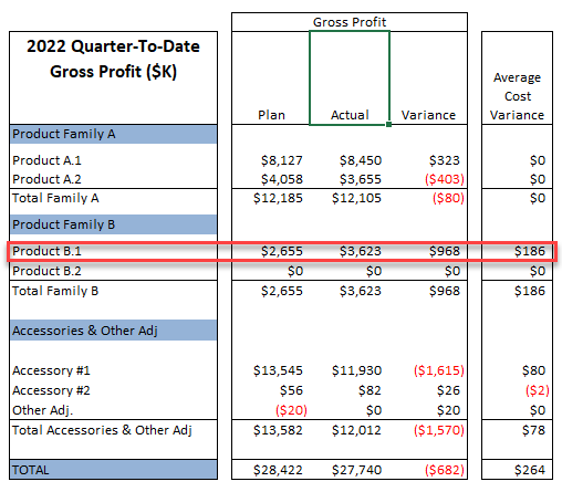
Below are the Average Cost Variances Product B.1 highlighted:
Same as above relative to Average Cost Variance, the 1Q plan vs. actuals for Product B.1 on our supporting schedules, the plan assumed that the business would ship 9,000 units @ $455/each for an extended cost of $4,095K. In actuality, the business shipped 9,700 units @ $436/each, totaling cost of $4,228K. Here’s the Average Cost Variance calculation for Product B.1:
Average Cost Variance = ($455 – $436) * 9,700 Units = Favorable $186K
Now we can state that the ASP variance of $59/unit ($750 plan vs. $809 actual), is so far the largest component of $968K variance at $575K favorable or 59%. Added to that is the $186K of favorable cost variance, totaling $761K or 79% of the total $968K variance. The Operations team must of worked some significant magic between when the plan was created, since they provided us with a $455/unit cost vs. today we are seeing a $436/unit cost, or a 4% cost reduction. Good job Operations Team!
Step #3 – Calculate Sales Volume Variance impact to Gross Profit
Plan vs. Actual volume variance affects gross profit through changes to revenue and costs. Generally, the more favorable the volume of units shipped, the more favorable the revenue variance and conversely the more unfavorable the cost variance, for obvious reasons. Here’s the formula for computing the Sales Volume variance:
Sales Volume Variance = (Actual Volume Shipped – Plan Volume Shipped) * Planned Unit ASP
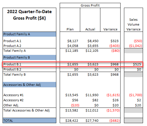
Below are the Sales Volume Variances for Product B.1 highlighted:
The Sales Volume Variance above is a favorable $525K, indicating the volume for Product B.1 was significantly higher in 1Q than planned. As we mentioned earlier, the 1Q planned volume was 9,000 units, while we were actually able to ship out 9,700 units in 1Q. The Sales Volume change is multiplied by the planned ASP, as follows:
Sales Volume Variance = (9,700 Act. Units – 9,000 Plan Units) * $750 Plan ASP = Favorable $525K
Up to this point we have a favorable $575K ASP variance, a favorable $186K Cost Variance and a favorable $525K Sales Volume Variance, totaling more than the total Gross Profit Variance we started with, which was $968K. I think we are going to have some bad news ahead, but so far Marketing is doing their job on Pricing, Sales is going their job by selling more units that we had planned and Operations was able to reduce unit prices a little. Let’s keep going on our quest.
Step #4 – Calculate Cost Volume impact to Gross Profit
As you would expect, if you have a favorable Sales Volume Variance as we do above, then you are going to have an unfavorable Cost Volume Variance because you are shipping a greater volume of inventory to customers. The variance is computed by multiplying the difference between the planned and actual units shipped, by the planned Average Unit Cost. Here’s the formula:
Cost Volume Variance = (Plan Volume Shipped – Actual Volume Shipped) * Planned Unit Average Cost
Below are the Cost Volume Variances for all the Products with Product B.1 highlighted:
In our example, there were 700 more units shipped than planned. The planned Average Unit Cost was $455, generating the following calculation:
Cost Volume Variance = (9,000 – 9,700) * $455 = Unfavorable $319K
As you can see above, shipping more than the planned unit volume results in a reduction to gross profit due to the higher volume of items being shipped to customers.
Step #5 – Calculate the Family-Level Volume Variance (or Final Volume) impact to Gross Profit
Next, we need to compute the Family-Level Volume variance, which will produce a slightly different result than summing the individual Product-Level Sales and Cost Variances. This is only applicable if your product hierarchy has summary groupings, which nearly every business has.
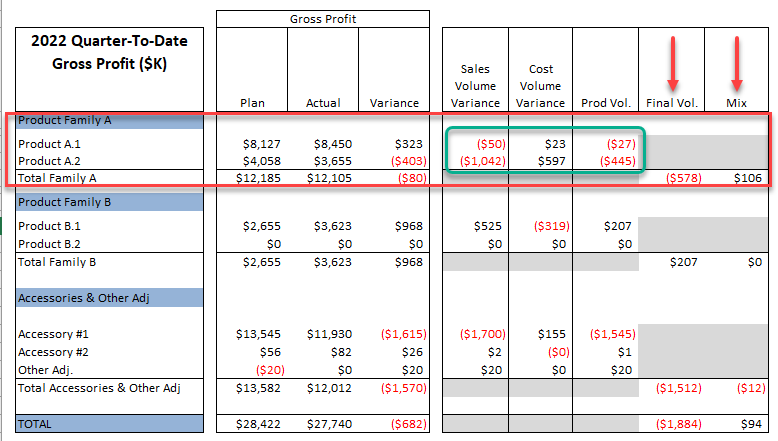
As you can see in our example below for Product Family A, there are two different products: 1) Product A.1; and 2) Product A.2. Both Products have their own plan, actual and variance. Product A.1 has a $50K unfavorable Sales Volume Variance and a $23K favorable Cost Variance, totaling $27K unfavorable. Product A.2 has a $1,042K unfavorable Sales Volume variance and a $597K favorable Cost Volume Variance, totaling $445K. Though it is not shown below, the total of Product A.1 and A.2 volume variances is an unfavorable $472K (Product A.1 $445K + Product A.2 $27K). That is helpful information, but we now need to compute the Final Volume Variance for Family A, which will produce a different result than summing Product A.1 and A.2 volume variances. Here’s the formula for computing the Final Volume Variance (note: FL stands for Family-Level):
Final Volume Var. = (FL Unit Gross Profit * FL Actual Units Shipped) – FL Total Plan Gross Profit
The Family-Level A Unit Gross Profit equals $790/Unit, actual Units shipped equals 14,700 and total planned Gross Profit equals$12,185K. Here’s the Final Volume calculation:
Final Volume Var. = ($790 * 14,700) – $12,185K = Unfavorable $578K
As you can see, the Family-Level A volume variance is a worse than if you only analyzed the individual products within the family. This is because there is a Mix component to the variance, which is our final calculation needed to reconcile the total variance for all products.
Step #6 – Calculate the Family-Level Mix impact to Gross Profit
The Mix Variance is applicable to the interaction between products within a group, or in our example a Family. It quantifies the impact of differences between individual products, with different proportional variances and gross profit amounts. Looking at the example above, you can see that the Product-Level Volume variances total $472K unfavorable, but the total Final Volume variance for Family A is $578K unfavorable, which reflects the Mix Variance.
You can either compute the Mix Variance by squeezing for the difference between the sum of the individual Product-Level Volume Variances and Subtracting the Family-Level Final Volume Variance ($472K Sum of the Family A Product Level Volume Variances – $578K Family-Level A Final Volume Variance = $106K Favorable Mix Variance) or compute the Mix Variance separately as follows (again FL is an abbreviation for Family Level):
Mix Variance = (Sum of Product-Level Plan Unit GP * Product-Level Actual Units Shipped for all products in Family) – (FL Actual Units Shipped * FL Plan Unit Gross Profit)
As can see, calculating the Mix Variance rather than squeezing for the Mix Variance is a bit involved, but the specific calculations/formulas are on the Excel template for your use. (Find out how to get your own copy of the Excel workbook used to generate this narrative along with the video instructions for nominal cost.)
Step #7 – Step back from the trees and gain some actionable insight
The expanded Gross Profit Analysis is displayed below.
Step #8 – Reviewing the Gross Margin Bridge results
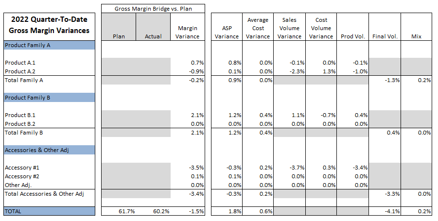
Finally, here are the gross margin variances that result from the earlier gross profit variances. All the margin variances are relative to the planned gross margin %, which in this case was 61.7%. The actual gross margin of 60.2% was calculated by dividing the actual gross profit ($22,740K) by the planned extended total sales ($46,102K), producing an unfavorable variance to plan of 1.5%. All the other gross margin variances are relative to the 1.5% unfavorable result.
This view is very helpful for understanding the scope of the impact in terms of margin differences. It becomes much clearer that the Accessory #1 is the main culprit in under achieving the company’s gross margin goals. The primary reason for missing the goal is a sales volume problem on that same product. Product Family B is producing strong results, primarily due to favorable ASP results (1.2%), followed by both some favorable volume (0.4%), and a slightly lower average cost for the total product family. Product Family A has a smaller unfavorable volume issue (1.3%) that is partially offset by good ASP results and some favorable mix performance. In conclusion, the focus should be: 1) figure out how to fix the Accessory #1 sales volumes, and; 2) work on Product A.2 volumes as well.
Step #9 – Purchase your own Gross Margin Analysis Tool Kit and expedite your efforts toward insightful margin analysis!
Get a copy of our Gross Profit/Margin Analysis Tool Kit workbook to ignite your company’s efforts to increased profitability and success. Here is what is included in the Tool Kit:
>
- Worksheet of your time phased sales plan (sales dollars, units and ASPs);
- Worksheet for your time phased cost of goods plan (cost of goods, units, unit costs);
- Worksheet for your time phased gross profit plan (gross profit dollars, gross margin, unit contribution dollars);
- Worksheet of your time phased sales actual (sales dollars, units and ASPs);
- Worksheet for your time phased cost of goods actual (cost of goods, units, unit costs);
- Worksheet for your time phased gross profit actual (gross profit dollars, gross margin, unit contribution dollars);
- Worksheet with the Gross Profit and Margin variances that includes an ability to easily change the period of review from a specific month, quarter or year to date; and
- Worksheet with some simple reporting tools to facilitate your analysis review.
- If you would like a copy of the Excel workbook used in the examples, please use the Contact Us button at the bottom of the page. Please feel free to leave comments and likes.
The Tool Kit is designed to analyze gross profit/margin variances against plan, but you can easily modify the template to perform the same analysis vs. prior year results too. Very nice!
FAQs:
Here are some common questions we get regarding Gross Margin Analysis:
- How do you build a gross profit plan? — If you would like detailed instructions on how to build a plan and get a free copy of the Excel model, see our How to Build a Time-Phased Sales and Cost Plan for Gross Margin Analysis blog post.
- Can I use this toolkit for prior year comparisons? — Yes! The templates are easily adaptable for year-over-year analysis. If you purchase the Tool Kit, we will also send you a copy of the updated version with the ability to perform prior year comparisons.
- Who is this Tool Kit for? — This is mainly intended for cost accountants, financial planning analyts and like, supporting midsize businesses. We are also working a more complex solution that leverages Power Pivot and Power BI to generate even more insightful gross margin analysis, such as year-over-year customer based analysis. Contact us if you would like to learn more.
Stop guessing about your margins-start driving results with data. Download your toolkit or training course today!
If you need assistance, we are available for consulting at reasonable rates. Contact us with any questions.


