Boost Inventory ROI and Service With Smart Strategies By Leveraging Our OptiStock Simulator
TABLE OF CONTENTS
- Introduction to OptiStock Simulator–An Inventory Optimization Tool
- What is a Statistical Inventory Simulation
- Scenario Model and Computations Explained
- How and Where All the Scenarios Are Recorded During Simulation
- How to Transform Your Inventory Management and Achieve an Optimized Balance of Customer Service, Inventory Levels and GMROI
- How to Obtain A Copy of The OptiStock Simulator Workbook To Boost Inventory ROI

Introduction to OptiStock Simulator — An Inventory Optimization Tool
Would you like to better optimize your inventory for both customer service as well as boost inventory ROI (aka Gross Margin Return on Inventory or GMROI)? How would you like to test different hypotheses around inventory replenishment to determine your best course of action before you issue another purchase order? If you would, then you have come to the right place to learn about our OptiStock Simulator, which is an inventory optimization tool that allows you test your inventory control hypotheses and see what happens. Generally speaking, inventory management is a function of balancing inventory levels and customer service, while also delivering an acceptable Gross Margin Return On Inventory (GMROI).
Achieving this balance requires understanding the impact of moving numerous inventory management levers, such as reorder points, safety stock, lead times, order up to levels, customer service assumptions, because many of them come with trade offs, hence the balancing act. In addition to balancing these trade offs, we need to understand the profitability of our inventory investment (GMROI again) and what impact these decisions are having on Cash Flow, to ensure corporate goals are achievable.
To increase the probability of achieving our corporate goals, we created OptiStock Simulator to run statistical simulations that will compute and record the results of as many inventory simulations as are required to understand the impact of changing those inventory levers and arrive at a reasonably optimized solution. For example, what happens to GMROI if we increase or decrease lead time one month or what happens to our probability of a stockout and/or if we reduce our customer service level preference from 95% to 90%. OptiStock Simulator will help you answer these types of questions and many more.
What is a Statistical Inventory Simulation?
A statistical inventory simulation is a quantitative method that uses a random number generator(s) to model complex systems, such as an inventory scenario, and evaluate the impact on of various inputs to generate a probable outcome. In this case, the random variable OptiStock Simulator will be generating is monthly shipment units or demand, using historical shipment trends to predict future demand. The important thing to understand is that using historical shipment trends to simulate future shipments is a common method for forecasting. It allows for the analysis of potential outcomes and their probabilities, thereby enabling better-informed decisions and risk assessments.
Before getting into simulation analysis, we will first go over the scenario model that is basis of an OptiStock Simulation.
Scenario Model User Inputs & Model Calculations
Scenario User Inputs
The example below is a snippet taken from the RopModel worksheet contained in the OptiStock Simulator Excel workbook.
Get a Free Copy of the Simulation Model Referenced Below, By Clicking Here
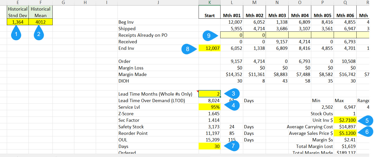
- Average Monthly Shipment Volume—The average monthly shipments which is computed by adding up all the units shipped over some period of time and dividing by the number of months in the sample. Or you can use Excel’s =AVERAGE(range) function
- Standard Deviation (Sample)—This is the average variation of the monthly shipments that are used to generate the Units Shipped random projection. Typically, you want 30 or more monthly shipments, without gaps, to get a reliable measure of variability. Given that we are making our projections from a sample of the shipment history population, we recommend using a sample standard deviation which is computed using Excel’s STDEV.S(range) function.
- Lead Time—This is the time required from placing a replenishment order to the time when the inventory is available for customer shipment, in months. Given our model is based on months, the Lead Time needs to be a positive whole number, from 1 to 6 months.
- Customer Service Level—This is the probability of having an item in stock when a customer order arrives. The Customer Service Level subtracted from one is the probability of a stockout. For example, a 95% Customer Service Level implies that there is a 5% probability of a stockout. The greater the Customer Service Level, the greater the amount of inventory required to achieve the Customer Service Level.
- Average Sales Price—This is the projected average unit sales price for each unit shipped.
- Average Unit Cost—This is the cost per unit that is used to calculate the inventory value on the balance sheet. When a unit is sold, this cost will show up as Cost of Goods on the income statement.
- Order Up To Level (OUL) Days—The OUL days is a measure of how much extra stock is needed to cover the gap between the time when an inventory item falls below a set reorder point and when a replenishment order for is placed with a supplier. The number of units is computed by dividing the Average Monthly Shipment Volume by 30 Days and then multiplying the daily shipment volume by the OUL Days. This can range from 0 days, assuming a replenishment order is replaced immediately after an item drops below its ROP, up to as many days as are required. Just remember that this increases the amount inventory required, just like increasing the lead time. More on this later.
- Month 0 Ending Inventory On Hand—This is just as it is described, which is the ending inventory as of the 0th month or Start month, which will become the beginning inventory amount for Month 1.
- Receipts Already On PO—In addition to the Start Month Inventory On Hand, any inventory that is already on PO and anticipated to be received in Month 1 or beyond, can be added to the model. If there is no inventory already on PO, the cells can be left blank
Scenario Model Calculations
The snippet below will help you understand what is being calculated in for each scenario given the Input Variables provided earlier.
Get a Free Copy of the Simulation Model Referenced Below, By Clicking Here
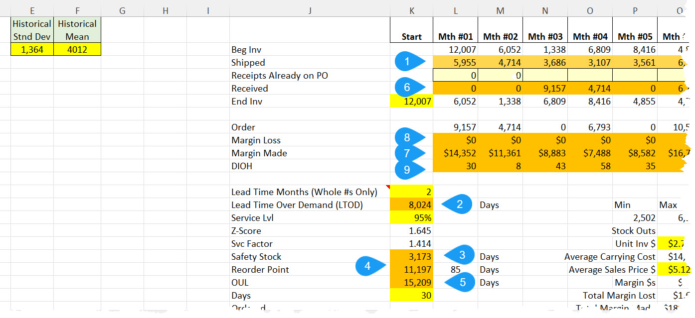
- Monthly Units Shipped—This key random variable, which is normally distributed and based on historical shipment volume and standard deviation, is generated separately for each month across the 18-month scenario. The Excel formula for computing the normally distributed random shipments values is as follows: =ROUND(NORM.INV(RAND(),Average Monthly Shipments,Sample Standard Deviation),0)
-
Lead Time Over Demand (LTOD)—LTOD is the number of units that will be sold in during the number of months of Lead Time. It is calculated by multiplying the Lead Time Months by the Average Monthly Shipment Volume.
- Safety Stock–Extra inventory held to prevent stockouts caused by uncertainties in demand or supply. It acts as a buffer to ensure that a business can continue to meet customer demand during unexpected delays or fluctuations, maintaining service levels and avoiding potential sales losses. It is computed using the service level, lead time and standard deviation. The higher the selected service level, the greater the amount of projected safety stock.
- Reorder Point (ROP)—The ROP is computed by combining the Lead Time Over Demand Units to the Safety Stock Units.
- Order Up To Level (OUL)—This is the ROP units from #4 plus the number of OUL days (User Input) multiplied by the daily average shipment volume. For example, assume an item has been depleted down to 1,000 units with a ROP of 1,100 and an OUL of 1,175. The part is now below the ROP; consequently additional stock is going to be ordered. To compute the amount to be ordered, subtract the OUL of 1,175 from the on hand stock of 1,000 to get the order quantity, which is 175 units in this example, assuming no other future replenishment orders.
- Units Received—Purchase orders are placed, using the established Reorder Point and OUL, and received using the established lead time (months). This represents the month in which a replenishment order is placed in stock.
- Margin Made—This is equal to the number of units shipped multiple times the per unit gross profit (Average Sales Price – Unit Cost).
- Margin Lost—When monthly demand exceeds on hand inventory, margin lost equals the units that could not be fulfilled times the unit gross profit. Generally, the higher the Customer Service Level, the lower the stockout units and associated Margin Loss. In the snippet below, there were no stockouts; consequently there is no Margin Loss.
- Monthly Days Inventory On Hand (DIOH)—This is the estimated number of days required to deplete the current month-end inventory based on the current average shipment volume
Scenario Model and Computations Explained
Scenario Model View
Snippet of a scenario on the RopModel worksheet, that is only displaying months #01 through #09 (the model computes 18 months for each scenario).
Get a Free Copy of the Simulation Model Referenced Below, By Clicking Here

Month-By-Month Computations Described
|
Period |
Activity |
|
Start Period (Mth #00) |
End Inv: This is where you input your most recent ME inventory units on hand. You can use a recent average of units on hand, but we recommend not leaving it 0 because you will have a stockout in Mth #01 which in all probability is not a likely event. |
|
Month #01 |
Beg Inv: 12,007 from the start month Shipped: 6,173 from the random normally distributed number generator Received: 0 received in Mth #01. If you anticipate receiving inventory in Mth #01, add it to the “Receipts Already on PO” row to immediately add inventory to stock. End Inv: The starting inventory of 12,007, less the 6,173 shipped leaves 5,834 on hand. Order: Given that the Ending Inventory is below the ROP of 11,197, then the model orders 9,375 (OUL 15,209 – 5,834 = The ROP is 11,197 with an OUL of 15,209. Given that nothing is already on order already, the model Orders 9,375 (15,209 less 5,834). Note that the model assumes a 2 month lead time, os you can see the 9,375 shows as a receipt in Mth #03. Margin Loss: There was no stockout; consequently, no margin loss. Margin Made: The Margin made is computed by multiplying the units shipped of 6,173 by the per unit gross profit of $2.41 (ASP of $5.21 less Unit Cost of $2.71) equals $14,877 of Gross Profit or Margin Made. DIOH: The Days of Inventory On Hand is just an estimate until we have 12 months of shipments at which time we use a rolling 12 month daily average of units shipped to divide into the ending units on hand. In Mth #01 we just divide the ending Units on hand of 5,834 by the units shipped of 6,173 divided by only 30 days to get an estimated 28 days of inventory on hand. |
| Month #02 |
Beg Inv: 5,834 from month-end Mth #01 Shipped: 4,933 random normally distributed shipment volume Received: 0 inventory received End Inv: 5,834 less the 4,933, with no received inventory produces 901 for the ending inventory balance. Order: As discussed in Mth #01, 9,375 was ordered and is expected in Mth #03, consistent with the lead time assumption—2 months. The 901 is below our ROP; consequently we need to look at ordering more, but this time we need to be cognizant of the Order we place in Mth #01. To compute the next order, we start with the OUL less the units on hand at the end of Mth #02 less what is already on Order or 15,209 – 901-9,375 = 4,933. You can see the 4,933 in the Mth #02 Order row. Margin Loss: $0 Margin Made: 4,933 times $2.41 = 11,889. DIOH: To compute the DIOH, we divide the ending units—901—by the daily average shipments for Mth #01 and Mth #02 ((6,173 + 4,933)/60 days = 185.10), producing 5 days of DIOH. |
| Month #03 | Beg Inv: 901 from month-end Mth #02
Shipped: 1,796 random normally distributed shipment volume Received: 9,375 from the Mth #01 Order arrived 2 months later End Inv: 8,480 = 901 Beg Inventory + 9,375 receipt – 1,796 Order: 0 No additional inventory was order because the 8,480 plus the outstanding Order from Mth #2 of 4,933, equaling 13,413 is higher than the ROP. Margin Loss: $0 Margin Made: 1,796 times $2.41 = $4,328 DIOH: To compute the DIOH, we divide the ending units—8,480—by the daily average shipments for Mth #01, Mth #02 and Mth #03 by 90 days producing 59 days of DIOH. |
| Month #04 |
Beg Inv: 8,480 from month-end Mth #0 Shipped: Random normally distributed shipment volume Received: 4,933 from Mth #02 Order received, per Lead Time assumption End Inv: 11,536 =8,480 + 4,933 receipt – 1,877 shipped Order: 0 because the 11,536 ending is still greater than the 11,197 ROP, but just barely Margin Loss: $0 Margin Made: 1,877 times $2.41 = $4,524 DIOH: To compute the DIOH, we divide the ending units—11,536—by the daily average shipments for Mth #01, Mth #02, Mth #03 and Mth #04 by 120 days producing 94 days of DIOH. |
| Month #05 |
Beg Inv: 11,536 from month-end Mth #04 Shipped: 5,899 random normally distributed shipment volume Received: 0 End Inv: 5,637 = 11,536 – 5,899 Order: 9,572 = 15,209 OUL – 5,637 Nothing already on Order in the next 2 months. Margin Loss: $0 Margin Made: 5,899 times $2.41 = $14,217 DIOH: To compute the DIOH, we divide the ending units—5,637—by the daily average shipments for Mth #01, Mth #02, Mth #03, Mth #04 and Mth #05 by 150 days producing 41 days of DIOH |
| Month #06
In this month we have a stockout. |
Beg Inv: 5,637 from month-end Mth #05 Shipped: 5,637 (the model actually called for 6,543, but we were constrained by available inventory; consequently, there was 906 units that went unfilled due to a lack of available inventory. Received: 0 End Inv: 0 Order: 5,637 = 15,209 OUL – 9,572 order in Mth #04 Margin Loss: 906 times $2.41 = ($2,183) Margin Made: 5,637 times $2.41 = $13,586 DIOH: Given the month-end inventory is 0 units, the DIOH is also 0. |
The above scenario continues on through 18 months, performing the same calculations as for the first 6 months described above. Below we discuss the scenario results.
Get a Free Copy of the Simulation Model Referenced Below, By Clicking Here

Inventory-Related Cash Flow Calculation Details
Above, we have hidden months 7 through 17 to display just the final totals. Notice that at point #1, we compute the cash flow generated for this scenario. The cash flow calculation is as follows:
1. Starting Inventory Cost: Start Inventory Unit Balance (12,007 units) multiplied by Unit Cost ($2.71) equals $32,539.
2. Ending Inventory Cost: Ending Inventory Unit Balance for Month 18 (4,466 units) multiplied by Unit Cost ($2.71) equals $12,103.
3. Cash Flow from Inventory Change: Subtract the Ending Inventory Cost from the Starting Inventory Cost ($32,539 – $12,103) to get $20,436 positive cash flow. This is positive because the inventory value decreased from the start month to the end month.
4. Margin Calculation: Add the Margin Made ($187,732) and subtract the Margin Loss (if any) to arrive at the total cash flow.
5. Cash Flow Calculation: Thus, the total cash flow over 18 months amounts to $208,168.
How and Where All the Scenarios Are Recorded During a Simulation
In the preceding example, we just completed one scenario using the User Input Variables. To better simulate real world results, we want to run our inventory scenario many, many times to minimize the impact of any outlier scenarios to produce a probable outcome. Each simulation starts with the blank template displayed below:
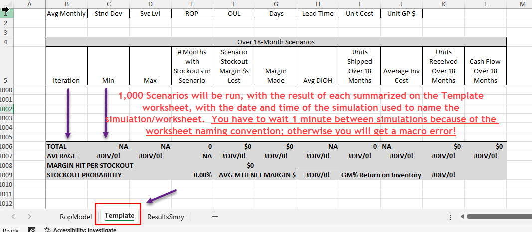
When requested, there is a macro that directs Excel to recalculate the entire scenario model, record the key results on the Template worksheet, and repeat for another 999 iterations.
Here’s the button you select to run the simulation, located on the RopModel worksheet:

Running an Inventory Simulation
First some background on the simulation
OptiStock Simulator will use an 18-month model to simulate one scenario, where assumptions for average historical monthly demand, the sample standard deviation for that demand, a service level assumption, a lead time assumption, days of additional stock for the OUL, unit Average Sales Price, unit Cost, starting inventory units on hand, and open purchase orders, if any. Each scenario will have 18 different monthly demand forecasts, that are normally distributed around the historical average monthly shipment history and associated standard deviation. The demand forecast and available inventory will be compared to the established reorder point and order up to level to simulate an actual inventory replenishment cycle. Depending on the key assumptions, there may be months with stockouts, as was shown in the earlier month-to-month example, which will be recorded along with the associated lost potential gross profit and units that were not fulfilled in a stockout month.
Once the “Run Simulation” button is selected, the simulation model will iterate 1,000 times over those same assumptions (this is the equivalent of pressing F9 to recalculate the scenario, 1,000 times) to get an average result. A Visual Basic macro is involved, which will record each of the 1,000 scenarios/iterations and summarize the results and assumptions on a separate worksheet for easy comparison, which you will most likely find very helpful when running a subsequent simulation. Once a simulation is complete, one or more variables can be changed to see how those changes impact stockouts, customer service levels, reorder amounts, average inventory level changes in both dollars and Days of Inventory On Hand (DIOH), and finally provide an Inventory Return on Investment (ROI) for that part. ROI is calculated by dividing an estimated annual gross profit (Average Monthly Gross Profit * 12 months) by the average inventory, for the 1,000 scenarios/iterations. This produces an estimated-annualized Gross Margin Return on Inventory as a percentage.
The Importance of GMROI to Inventory Analysis
Though OptiStock Simulator produces many performance metrics, GMROI is probably the most important. As explained above, OptiStock Simulator calculates GMROI by dividing an estimate of the annualized Gross Profit by the Average Monthly Inventory value. For example, let’s assume that a simulation results in an Average Monthly Gross Profit of $1,300, multiplied by 12 months produces an annual estimated Gross Profit of $15,600. Additionally assume that the simulation has an Average Monthly Inventory Dollar amount of $2,200. This would produce a GMROI of 709% ($15,600 / $2,200). This indicates that, on an annual basis, every dollar of invested inventory, is producing $7.09 of gross profit. Unfortunately as you will find, just increasing the inventory investment is not going to increase the GMROI, it will only dilute margin, assuming the average shipment volume remains unchanged. Things that will improve the GMROI include reducing the Customer Service Level, decreasing the lead time and/or days OUL. Additionally, increasing the ASP and/or decreasing the average unit cost, will also help improve GMROI. But all these tweaks come with some countervailing offset, such has higher probabilities of stockouts, which go hand in hand with lower service levels; consequently you will need to be selective when analyzing how to increase GMROI.
Starting a Simulation
Once the Run Simulation button is selected on the RopModel worksheet, the VBA macro creates a new worksheet and begins iterating and summarizing each of the 1,000 scenarios on a separate worksheet. At the end of the simulation, OptiStock Simulator summarizes the simulation results on another worksheet named ResultsSmry.

Worksheet Summarizing 1,000 Scenarios
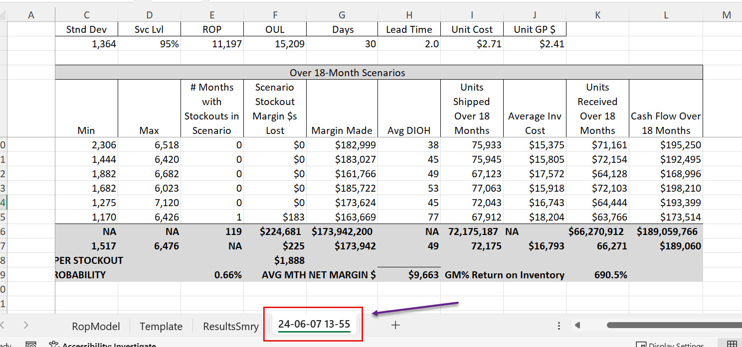
Given that all the important results above are summarized on the ResultsSmry worksheet, we will explain what all the above means in due course. The key is noting that the new worksheet is titled “24-06-07 13-55”, indicating that this simulation was run on June 7, 2024 at 1:55 PM. A limitation to the macro is that it can only be run once per minute because of the worksheet naming convention.
Analyzing an OptiStock Simulation Result
Once the simulation has iterated the 1,000 scenarios, in addition to documenting the result at the bottom of the newly created worksheet (24-06-07 13-55 in this case), the results are also summarized on the ResultsSmry worksheet. A snippet of the simulation results is as follows:
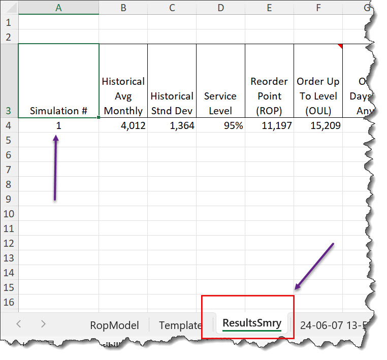
Above you can see that we are now viewing the ResultsSmry worksheet, with the simulation number referenced in column A on the ResultsSmry worksheet. Though not all the columns are referenced above, here is the information that is logged for each simulation in column order:
| ResultsSmry Column | Description |
|---|---|
| Simulation # | This is the simulation number. You can modify an assumption, such as changing the Service Level and rerun the simulation. The subsequent result will be simulation #2, and so on and so forth. Below the “Run Simulation” button is a button that will clear all the data on the ResultsSmry worksheet. |
|
Historical Avg Monthly |
This is the monthly average units shipped metric input on the RopModel page. More on this later. |
|
Historical Stnd Dev |
This is the sample standard deviation for the monthly average units shipped data set. |
|
Customer Service Level
|
Again, this is the probably of not having a stockout. One minus the Customer Service Level is the probability of a stockout |
| Reorder Point (ROP) |
The ROP used to determine when to order more stock. |
| Order Up To Level (OUL) |
The OUL used to determine how much stock to purchase (OUL – Stock On Hand = Replenishment Order) |
| OUL Days (If Any) |
The number of days used to compute the OUL. If the number of days is 0, then the OUL equals the ROP; otherwise, the Average Monthly Units Shipped is used to determine a daily amount of units shipped, assuming a 365 day calendar. This amount is multiplied by the OUL Days and added to the ROP to get the actual OUL number. |
| Lead Time (Months) |
Time required from the day a replenishment order is placed to the day it is received as new stock. |
| Item Unit Cost |
The Unit Cost used to compute the total inventory component value. This is also the cost used to relieve Inventory when a unit is shipped, that is reflected as Cost of Goods Sold. |
| Item Unit Gross Profit $ |
Per unit gross profit calculated by subtracting the Unit Cost from the Average Unit Sales Price (ASP). |
| Avg Monthly Min | The minimum units shipped is recorded for each 18-month scenario that is run. This is the average minimum for all the 1,000 scenarios. |
| Avg Monthly Max |
The maximum units shipped is recorded for each 18-month scenario that is run. This is the average maximum for all the 1,000 scenarios. |
| Avg Monthly Shipped |
The average monthly units shipped for all 1,000 scenarios which is comprised of 18,000 months (18 months per scenario) |
| Total # Months with Stockouts |
This is the number of months that experienced a stockout from the 18,000 months simulated. |
| Probably of Stockout in Any Given Month |
This is the Total # Months with Stockouts divided by 18,000 (the number of months simulated) |
| Avg Monthly Stockout Units |
In the event there is a stockout month, this is the average number of units that will be shorted in a stockout month. |
| Avg Monthly Gross Profit $s Lost to Stockouts |
If there is a stockout, this is the average gross profit foregone or lost due to the stockout. It is just the units shorted by the gross profit per unit shorted. |
| Avg DIOH |
This is an average of averaged in that each scenario has an average DIOH, that is the average over the 18-month scenarios. This is the average of the 1,000 scenario averages. |
| Avg Monthly Inv. Dlrs |
Each scenario has a computed average monthly inventory value, which is the average over the 18-month scenario. This is average over the 1,000 scenarios in the simulation. |
| Avg Monthly Revenue |
This is the Average Monthly Revenue for all 18,000 months (1,000 iterations * 18 months). |
| Avg Monthly Gross Profit |
This is the Average Monthly Gross Profit for all 18,000 months. |
| Gross Margin Return On Inventory (GMROI) |
This is the annualized gross profit divided by the average $s of inventory on hand over the 18,000 months. |
| Average Cash Flow Over 18-Month Scenario |
Computed by subtracting the beginning inventory value at the Start period minus the Mth #18 inventory value, which is the change inventory values, plus the gross profit for all 18 months of each scenario. If you want a number that is closer to annual cash flow impact, divide this number by 1.5. |
|
Worksheet Name |
Name of the Simulation worksheet in the YY-MM-DD HH:MM format described earlier. |
How to Transform Your Inventory Management and Achieve an Optimized Balance of Customer Service, Inventory Level and GMROI
The real power of simulation is changing your assumptions and then running another simulation to compare the results, which helps you understand the impact of tweaking the different User Variables. Below we will walk you through what is required to get begin optimizing your own inventory situation and gain control over your most important asset.
How to Compute The User Input Variables
As an example, we will use three sets of Input Variables and compare the results. But first, we need to collect historical data relative to Average Monthly Shipments, Average Sales Prices, Average Unit Cost and the standard deviation of the unit shipment volumes. If possible, you will want to collect 30 or more data points (separate monthly shipments) to produce more realistic simulations. If you have to utilize fewer data points, the sample standard deviation is going to be greater than it might otherwise be, leading to higher variability in the model than what may be experienced in the real world.
We have built a simple Excel workbook to collect month shipment results, which appears as follows:
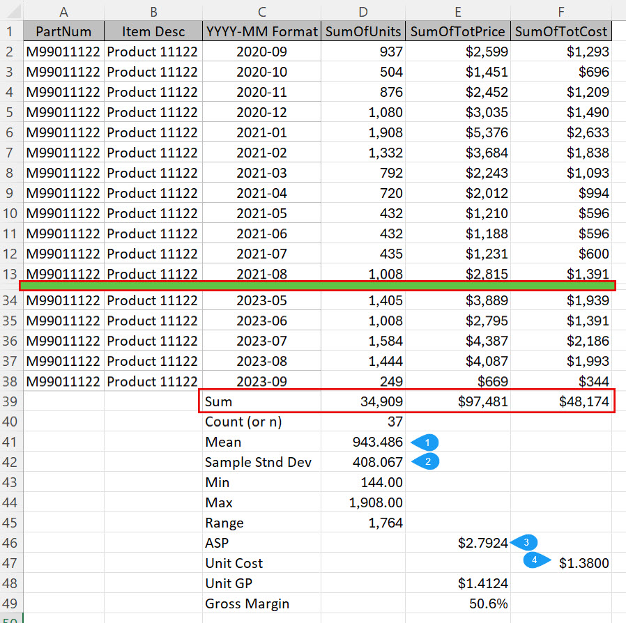
Above, we have retrieved the past 37 months of shipment history (September 2020 through September 2023 in the YYYY-MM Format for dates), including the units shipped (column D), invoiced total (column E) and cost of goods (column F), which is summarized in row 39. The worksheet is available for free if desired and summarizes the necessary variables, including: 1) mean or average monthly shipments (943 units per month); 2) the sample standard deviation of 408 units, computed using Excel’s sample standard deviation function (=STDEV.S(D2:D38)); 3) the Average Unit Sales price of$2.7924; and 4) the Average Unit Cost of $1.3800. Additionally, we were able to ascertain that our business had 1,850 units on hand as of month-end September 2023, with another 1,100 units on order and expected to be received in Mth #02. These values will be input on the RopModel worksheet.
Shipment Data Normalcy Assumption Explained
As we said before, we assume that the shipment data follows a normal distribution with a mean. If we make a histogram using the 37 shipments above, we can see that the shipment amounts seem to follow a normal distribution:
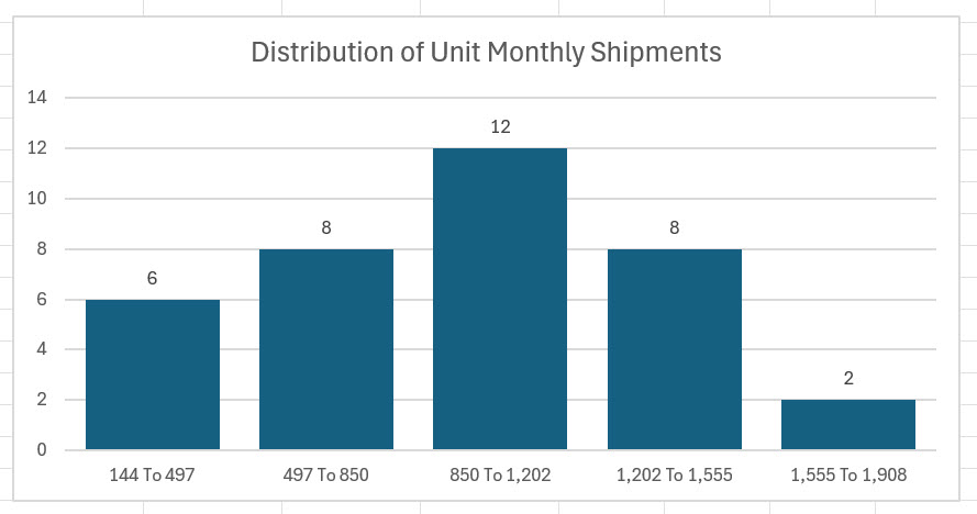
You can use the histogram function in the worksheet that calculates the Input Variables, to check the data visually. There is also a statistical test for how well the shipment data fits a normal distribution (aka Goodness of Fit), but it is beyond the scope of this already long post. You can search for it on Google, if you want to learn more about testing your data for the Normal Distribution.
Calculated Scenario/Simulation Constants
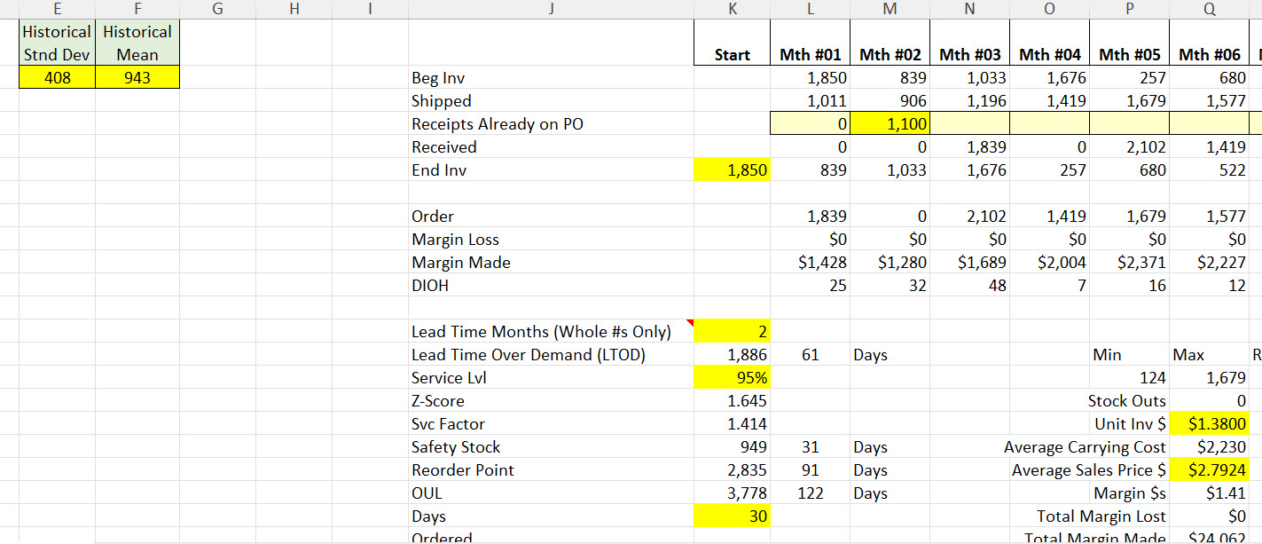
With the Input Variables established, we can see the calculated constants that will be used for the baseline simulation, including the following:
- Lead Time Over Demand (LTOD)—Given that we used a 2-month lead time assumption, the LTOD units are 2 times the monthly average unit shipment of 943 = 1,886 units;
- Safety Stock—Safety stock formula is the Svc Factor (or the square root of lead time) 1.414 * sample standard deviation 408 * the Z score for 95% service level 1.645 = 949 units.
- Reorder Point (ROP)—This is LTOD 1,886 + Safety Stock 949 = 2,835.
- Order Up To Level—In this first iteration, we are using a 30-Day assumption for our OUL level, which is computed by adding to the ROP of 2,835, another 30 days of unit demand (943 Monthly Average * 12 Months / 365 Days * 30 Days OUL = 3,778
The graphic below displays both the initial Input Variables and the resulting constants described above:
Get a Free Copy of the Simulation Model Referenced Below, By Clicking Here
Running the Simulation Model and Interpreting Results
You can run as many simulations as you want, but we will only run three different ones to see how our changing assumptions affect cash flow, GMROI and stockouts. The stockout definition is when we do not have enough stock to meet the forecast monthly demand, represented in both lost units and gross profit. But you should note that the cost of stockouts can hurt by more than just lost gross profit. For example, if we disappoint a big customer too often, they may look for another vendor. So we need to think carefully about the cost of stockouts beyond just the lost gross profit to fully realize the financial impact of stockouts, including lost goodwill.
In our hypothetical example, we want to better understand the impact of changing both the Order Up To Level Days and Service Level assumptions. By policy, in our example we utilize 30 days to increase the Order Up To Level and set the customer service level at 95%; consequently, simulation #1 is going to use a 95% Customer Service and an OUL Days assumption at 30 days. For simulation #2, we will decrease the OUL Days from 30 to 15. And finally, simulation #3, we will change the OUL Days back to the 30 days used in simulation #1, but now decrease the Service Level from 95% to 90% and then compare the results.
Summary of The Input Variables Used For All 3 Simulations
| Input Variable | Simulation #1 Baseline Model | Simulation #2 Reduce OUL By 15 | Simulation #3 Reduce Customer Svc Level by 5% |
|---|---|---|---|
| Monthly Average Shipment Units | 943 | 943 | 943 |
| Sample Standard Deviation | 408 | 408 | 408 |
| Lead Time (Months) | 2 | 2 | 2 |
| OUL Days | 30 | 15 | 30 |
| Customer Service Level | 95% | 95% | 90% |
| Avg Sales Price | $2.79 | $2.79 | $2.79 |
| Avg Unit Cost | $1.38 | $1.38 | $1.38 |
| Starting Inventory Quantity On Hand | 1,850 | 1,850 | 1,850 |
Resulting Simulation Analytics
| Input Variable | Simulation #1 Baseline Model | Simulation #2 Reduce OUL By 15 | Simulation #3 Reduce Customer Svc Level by 5% |
|---|---|---|---|
| Monthly Average Shipment Units | 943 | 943 | 943 |
| Sample Standard Deviation | 408 | 408 | 408 |
| Customer Service Level | 95% | 95% | 90% |
| Reorder Point (ROP) | 2,835 | 2,835 | 2,625 |
| Order Up To Level (OUL) | 3,889 | 3,307 | 3,568 |
| OUL Days | 30 | 15 | 30 |
| Lead Time (Months) | 2 | 2 | 2 |
| Item Unit Cost | $1.38 | $1.38 | $1.38 |
| Item Unit Gross Profit $ | $1.41 | $1.41 | $1.41 |
| Average Monthly Min (Units) | 226 | 226 | 230 |
| Average Monthly Max (Units) | 1,676 | 1,676 | 1,668 |
| Average Monthly Shipped (Units) | 941 | 939 | 943 |
| Total # Months With Stockouts | 173 | 197 | 192 |
| Probability of Stockout in Any Given Month | 1.0% | 1.1% | 1.6% |
| Average Monthly Stockout (Units) | 230 | 162 | 251 |
| Average Monthly Gross Profit $s Lost to Stockouts | $324 | $228 | $354 |
| Average DIOH (Days) | 56 | 48 | 49 |
| Average Monthly Inventory $s | $2,212 | $1,866 | $1,951 |
| Average Monthly Revenue $s | $2,627 | $2,622 | $2,633 |
| Average Monthly Gross Profit $s | $1,329 | $1,326 | $1,332 |
| Gross Margin Return On Inventory (GMROI) | 721% | 853% | 819% |
| Avg Cash Flow Over 18-Month Scenario | $23,163 | $23,641 | $23,630 |
| Worksheet Name | 24-06-12 10-50 | 24-06-12 10-51 | 24-06-12 10-52 |
How To Interpret OptiStock Simulator Results
Above we have highlighted the most material changes driven by the tweaks we made in Simulations #2 and #3.
- Service Level: You can see that the service level was constant, at 95% in Scenarios 1 and 2, but decreased to 90% in #3. You can see the impact in both DIOH and Avg Monthly Inventory.
- : Reorder Point: The ROP dropped in #3 because of the drop in service level. This decreased the safety stock 210 units. Later you will see that the number of stockout increases accordingly.
- Order Up To Level (OUL): The OUL was impacted in #2 by the decrease in OUL days and #3 by the decrease in Customer Service Levels. Decreasing the OUL days had a bigger decrease in OUL units than decreasing the Customer Service level.
- Probability of Stockout in Any Given Month: This increased from 1.0% in #1, to about 1.1% in #2 and 1.6% in #3; consequently, it appears that decreasing the Customer Service Level has a greater impact on stockouts than dropping the OUL days 50%.
- Avg Monthly Stockout Units: Though it is a bit counterintuitive, the Stockout units dropped from #1 to #2. We may want to run this simulation a couple of more times, but the displayed result is based on 1,000 scenarios; consequently, it is more than likely solid. The #3 simulation did increase to 251. Again, this number represents the expected number of shorted units given a stockout. If there were an average order size, we could determine how many orders would be shorted which would help provide a more realistic cost of a stockout beyond just the lost gross profit.
- Avg Monthly Gross Profit $s Lost to Stockouts: Again, because the average units shorted decreased in #2, the gross profit lost to stockouts decreased when we decreased the number of OUL days.
- Avg Monthly Inv. Dlrs: Decreasing the OUL Days by 15 in #2 had a bigger impact to reduce inventory than reducing the Safety Stock from 95% to 90. In #2, average inventory on hand decreased from a month average of $2,212 to $1,866 (16%) vs to $1,951 (12%) in #3.
- Gross Margin Return On Inventory (GMROI): This is where you can really see a financial difference in that #1 was 721%, which indicates that for every $1 of inventory investment, there is $7.21 in annual profit. That increased to $8.53 (18% improvement) in #2 and $8.19 (14% improvement) in #3.
Simulation Review And Conclusions
From the results above, it appears that decreasing the OUL days in #2 had a greater impact on profitability than decreasing the customer service level. This can especially be seen in the change in the GMROI metric. Though this could use additional review and analysis, analyzing various inventory parts, depending on profitability, lead time, customer service sensitivity will pay huge dividends when assessing operational policy around inventory replenishment. For example, you can determine what would be the impact of switching vendors that have shorter lead time, but are slightly more expensive. You could run a number of simulations to determine who much profit could you give to gain a month of lead time, and simultaneously reduce inventory dollars, to get the same GMROI or better. There is a fairly endless list of ways to test different inventory improvement hypotheses to improve the likelihood of overcoming challenging barriers with respect to inventory management.
How to Obtain A Copy of the OptiStock Simulator Workbook To Boost Inventory ROI
There are currently two separate versions of OptiStock Simulator workbook. There is a free version (OptiStock Simulator Basic), that is the equivalent of what was described above where you have complete freedom to modify the User Input Variables. All other variables are protected as is access to the Visual Basic code. In addition to the Basic version, there is an Advanced version. In the Advanced version, you have the freedom to modify the entire workbook, including the Visual Basic code. OptiStock Simulator Advanced is available at Profitwyse Academy for $75.00 as is the free Basic version. Also, if you would like assistance with modifying the Advanced workbook, you can purchase consulting time, in 30 minute increments, for $65.00 each, also available at Profitwyse Academy.
BONUS! Looking for an Efficient Solutions to Plan Your Daily Cycle Counts?
Check out the YouTube video below to learn you to simplify and streamline your periodic daily cycle count planning process. Here’s
Establish Your ABC Coding Strategy
The tool has a worksheet where you list all the inventory items you want to cycle count, providing fields for Part ID, Description, Assignment Criteria and ABC Code categorization. The Assignment Criteria column can contain whatever metric you would like to utilize when determining whether a Part ID is going to be an A, B or C part, e.g. units shipped, units manufactured, units consumed, or whatever works for your organization. Given your Part IDs, count frequency assumptions for A, B and C parts, the tool will compute the total number of counts you will need in a given year to fully comply with your preset cycle counting objectives.
Establish Your Cycle Count Calendar
Given that the cycle count planning tool is going to assign Part IDs to be counted on predetermined days, you have to specify the following: 1) days of the week your staff will be cycle counting (or not, such as Saturday and Sunday). If needed, you can elect to cycle count 7 days a week but typically it will be Monday through Friday. Additionally you can omit a weekday for the counts, e.g. no counts on Fridays. You will also need to input you holiday schedule if you are not going to be counting on Christmas Day (assuming it falls on a weekday). You can set 20+ holidays or other dates (such as a pre-planned all hands meeting where no cycle counting will be performed). Once you have set you calendar, there is a Build Calendar button where a macro will build out your cycle count calendar with all the dates that cycle counting will be performed.
Generate Your Daily Cycle Count Plan
Once you have set your ABC coding and cycle count calendar, you can push the Build CC Plan button, which will initiate a VBA program that randomly slots each part in a cycle count plan that aligns with your specifications for A, B and C part count frequencies. The result will be written to an Excel Table, with the planned count date and Part ID to be counted on that date for the time period specified, typically a year. Saving the cycle count daily plans to an Excel table makes it very easy for whomever is administrating the cycle plan to just filter for a month, print the data and send it off to the cycle count team for execution.
Check Out The YouTube Video Below for Additional Details/Demonstration
Get more information and/or request your copy of the Cycle Count Plan tool.
Hopefully you found this enlightening and can utilize it in your own organizations. We have the tools to help.

