Empowering Your Sales Team: Business Analytics Strategies for Success

 

As financial and accounting mavens within the organizations we serve, the value we can bestow on other functions cannot be understated.  This especially applies to the Sales Team.  That said, our Sales Team partners are not always the most sophisticated users of business analytics; consequently, we need to find applications of business analytics that are easily digestible and drive sales growth.

Finding applications of business analytics for your Sales Team necessitates an ability to bridge the gap between what can be complex data insights and the need to distill those insights into practical sales strategies.  With this goal in mind, your efforts will lead to tangible and meaningful analysis that empowers the Sales Team moving forward.

In this article, we are going to cover an application of Excel to create some novel business analytics, using a couple of Excel’s statistical functions, to achieve our goal of bringing meaningful insights to the Sales Team.  We will make use significant use of the Normal Distribution, and its characteristics, to create a tool that, on an individual product basis, will provide each Sales Rep with a metric that provides the probably of each customer consuming their last unit one week, two weeks, three weeks and four weeks out from the date of the report.   

Business Analytics Strategies That Leverage The Normal Distribution

Before you go too far, let’s discuss the problem and solution.  As mentioned earlier, we want a report that can be emailed to our Sales Reps on a monthly basis that will give them some insight into what is being shipped to the customers residing in their territories.  In addition to this basic information, we also want to provide some insight into the probably that a given customer has exhausted their most recent receipt of each our products.  To this end, we want to show the sales rep the probably of Product XYZ being exhausted one week from the date of the report, as well as two, three and four weeks out from the date of the report.  Here’s what our completed report looks like for (sorry but this needs to be viewed on a desktop browser).

Consumption Analysis Report Example for Jerry Jones

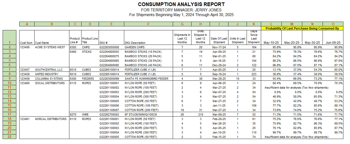
The above Consumption Analysis Report, that includes only customers assigned to Jerry Jones (our fictitious Sales Rep), is utilizing all shipments from May 1, 2023 through April 30, 2024, as example for the one Sales Rep. 

Column	Description
A & B	Customer Number and Name
C & D	Product Hierarchy Number and Title
E & F	Part Number and Description
G	Number of shipments in the prior 12-month period (in this case May 1, 2023 through April 30, 2024)
H	Quantity of units shipped in the prior 12-month period
I	Date of most recent or last shipment
J	Quantity of units in the last or most recent shipment
K	Days since the last or most recent shipment.  This can be computed by subtracting the date of the most recent shipment at column I, from the end date of the current report–April 30, 2024–to derive the number of days between the two dates.
L	Probability of last or most recent shipment being fully consumed 10 days past the end date of the current report.  Given the end date of the current report is April 30, 2024, then 10 days past that date is May 10, 2024.
M	Probability of last or most recent shipment being fully consumed 20 days past the end date of the current report–May 20, 2024
N	Probability of last or most recent shipment being fully consumed 30 days past the end date of the current report–May 30, 2024
O	Probability of last or most recent shipment being fully consumed 40 days past the end date of the current report–June 9, 2024

Here is Why This Report Is Valuable

The purpose of this solution is to enhance the Sales Rep’s ability to examine each customer and product individually, enabling them to identify products that each customer may need to reorder, potentially even before the customer recognizes the need. Isn’t that powerful knowledge? We certainly believe so!

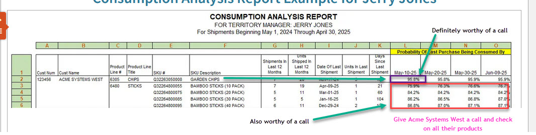
For instance, let’s examine row #2, which pertains to Customer Acme Systems West. The first product listed, Garden Chips, shows a 96% probability of being consumed (or sold, if acting as a distributor) by Acme Systems West. Given Jerry Jones’ demanding role as a Sales Rep, he must prioritize his customer interactions on May 10th. If Acme Systems West has a 96% probability of having exhausted their stock of Garden Chips, a phone call would be warranted. Additionally, several of the Bamboo Sticks also exhibit high consumption probabilities. Jerry should get in touch with the buyer at Acme Systems West and prompt them to assess their inventory of these products.

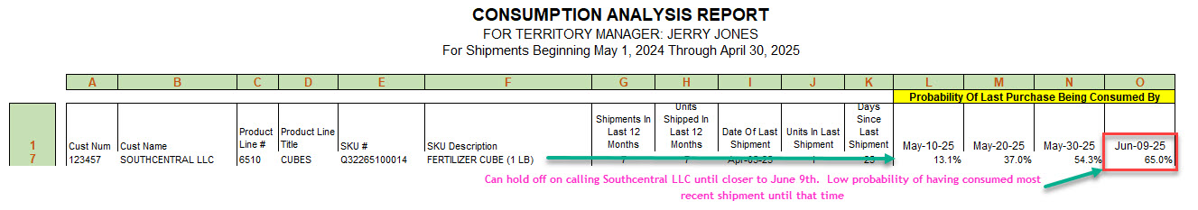
Moving on to rows 7 and 8, Jerry notices a low likelihood of Southcentral LLC using their recent shipment of Fertilizer Cubes (13% probability), as well as United Industry with the same item (37% probability).

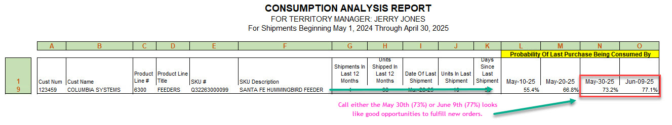
Row 9 presents the situation with Columbia Systems, who are approaching the depletion of their latest purchases of Santa Fe Hummingbird Feeders. With a 55% probability as of May 10th, he might choose to wait another 20 days when the likelihood of Columbia Systems having utilized their last Santa Fe Hummingbird Feeder exceeds 70% probability.

Imagine if each Sales Rep managed 40 to 50 customers, each averaging 10 products from our hypothetical company. This would mean overseeing nearly, or even more than, 500 distinct products that the Sales Rep must track to achieve their sales targets. The report is straightforward to comprehend and is devoid of the statistical complexities needed to calculate the probabilities. If you were a newly hired Sales Rep, you could efficiently grasp the circumstances surrounding our customers and their product purchases by utilizing a report similar to the one provided above.

What is the Normal Distribution and How Does It Help Forecasting Events?

If you need to forecast events, or know the probability of an event, then understanding the Normal Distribution and how it is used to forecast events is going to be important.  First we will review the normal probability distribution and then how it relates to Excel’s NORM.DIST() function, which is where we get our probabilities.  A discussion of the normal probability distribution begins with continuous random variables.  Examples of continuous random variables include: i) measurements of time needed to perform a job; ii) the time required before something fails, such as a tool, or tire, or whatever.   Any random variable whose values are measurements, as opposed to counts, is a continuous random variable.  Without too much discussion, suffice it to say that in nature, continuous random variables have a frequency distribution that approximates a bell-shaped curve or, as is known in statistical terminology, a normal probability distribution; consequently, we can leverage the normal probability distribution in our efforts to predict when our customers have exhausted their most recent product shipment.  The normal probability distribution, with a mean (μ) of 0 and standard deviation (σ) of 1, including the area included at +/- 1, 2 and 3 standard deviations from the mean, appears as follows:

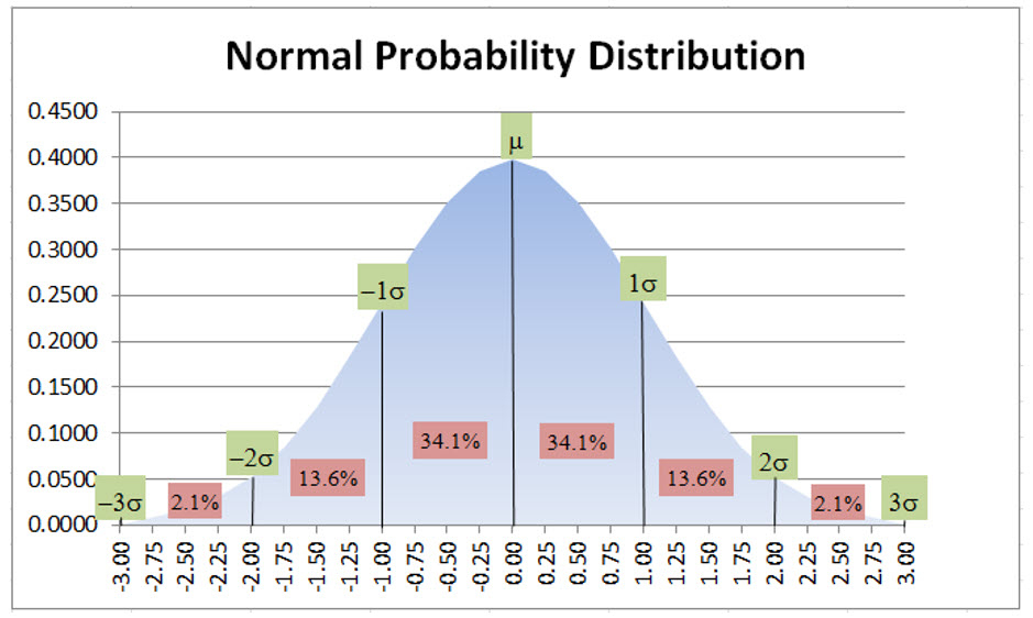
The basic characteristics of the normal probability distribution are that 68.2% of the observations occur within +/- 1 standard deviation of the mean (34.1% + 34.1%), and 95.4% occur within +/- 2 standard deviations and essentially 100% are within +/- 3 standard deviations.  Given that many, many continuous random variables, within a sample, are normally distributed, we can extrapolate the normal distribution characteristics to various forecasting problems using Excel’s NORM.DIST() and NORM.INV() functions.  If you need a refresher on how to utilize the normal distribution when determining the probability of various events, there are numerous YouTube videos, including Normal Distribution Word Problems, from Steve Crow, that are good refreshers. 

Hopefully you found that helpful.  One of the things that the author does in this video is to utilize Normal Probability Distribution tables.  These are standardized tables, with a mean of 0.0 and standard deviation of 1.0, that can used to look up probabilities based on Z scores (author shows how to compute Z scores).  To utilize the table, you have convert your test statistics into a Z score.  In our example, we are going to use the power of Excel, which eliminates the need to convert test statistics into Z scores and manually look up probability distributions in a table, which is our application would be impossible. 

Leveraging Microsoft Excel’s NORM.DIST() and NORM.INV() Functions in Your Strategic Business Analytics Applications

If you watched the Normal Distribution Word Problem YouTube video above, which is extremely helpful in understanding how normal distribution probabilities are applied to business problems, you will note that computing Z scores and looking up Standard Normal Distribution values in a table is a rather cumbersome process.  Our application is going to take advantage of Excel’s NORM.DIST() and NORM.INV() functions so that we can can efficiently compute thousands and thousands of test statistics in our application. 

How to Use the NORM.DIST() Function

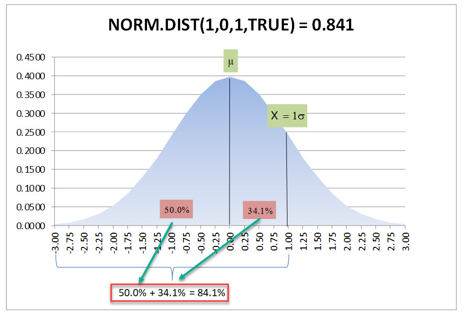
Reviewing Microsoft’s definition of the NORM.DIST() provides definitions of the following four arguments: 1) X or the value for which we are seeking a distribution (we will discuss the X in more detail momentarily); 2) distribution mean; 3) distribution standard deviation; and 4) a logical value, that if TRUE returns the cumulative distribution function.  Just as an example using the Standard Normal Distribution table displayed above, if we plugged in a test statistic of 1.0, a mean of0.0 a standard deviation of 1.0, and TRUE for the Cumulative option, our NORM.DIST() would return the area from the far left of the curve, starting at 0 moving toward the mean, which is 50% of the area under the curve, plus 1.0 standard deviation to the right of the mean is another 34.1%, resulting in 84.1% or:

NORM.DIST(1.0,0,1.0,TRUE) =  0.841

Graphically, this is the area under the curve that the above NORM.DIST function is attempting to capture:

How to Use the NORM.INV() Function

As you might have suspected, the NORM.INV() function is the inverse of the NORM.DIST() function, in that it will give you the test statistic or X when you provide other parameters.  Looking at the Microsoft Excel description for the NORM.INV() function, there are only three parameters required, which are as follows: 1) Probability; 2) Mean; and 3) Standard Deviation.  To illustrate the inverse nature of this function, we will invert the inputs from our earlier example:

NORM.INV(0.841,0,1.0) =  1.000

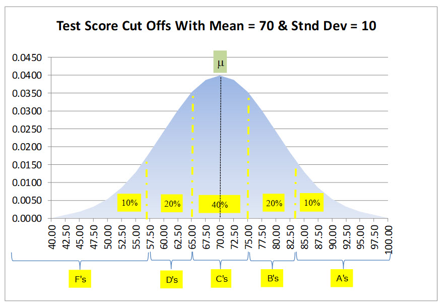
How about an example that we can all relate to—a test given to 30 students?  On our test, the maximum score was 100 points, the mean (or average) score was 70 points, with a standard deviation of 10 points.  Rather than the usual 70 to 79 points is a “C”, 80 to 89 is a “B”, etc., our instructor wants to use statistics to determine the grading scale.  He has decided that 40% of the students will receive a “C”, 20% a “B”, 10% an “A”, 20% a “D” and 10% an “F”. 

First we will determine how to get the “C” grades.  Since we want 40% of grades to be a “C” we need 20% on both sides of the mean, which is 70 points in this example.  We can use the NORM.INV() function to give us this value.  Remember that NORM.INV() is looking for  the cumulative distribution percentage from X= 0 to the X value we are seeking. So we provide 70% to the function which will give us the X value that corresponds to the cumulative proportion or percentage, along with filling in the respective mean and standard deviation, which is as follows:

NORM.INV(0.70,70,10) = 75.24 points

Subtracting our mean of 70 points tells us that 5.24 points will capture 20% of the test scores to the right of the mean or stated differently 20% of the students are expected to score from 70 to 75.24 points.  Subtracting the 5.24 from our 70 point mean gives the 20% below the mean, which is 64.76, and provides the 40% range for the “C” grade (scores from 64.76 to 75.24 receive a “C” grade).  To determine the area for grades “B” and “D”, which encompasses the next 20% beyond our “C” range, we can just calculate the difference between the area at 90% and 70% as follows:

NORM.INV(0.90,70,10) – NORM.INV(0.70,70,10) = 7.57 points

Using the top “C” grade of 75.24, we now can state that everyone scoring from 75.25 to 82.82 (75.25 + 7.57 for the next 20%) will receive a “B”.  Conversely, anyone scoring lower than 64.76 to 57.18 (64.75 – 7.57 for the next 20%) will receive a “D”.  Finally, anyone with a score greater than 82.82 will receive an “A” and lower than 57.18 will receive an “F”.  Summarizing our result we get the following table:

Grade	Rounded Test Score (S)	Target % of Students Receiving Following Grade
A	S > 83	10%
B	75 < S <= 83	20%
C	65 < S <= 75	40%
D	57 < S <= 65	20%
F	S <= 57	10%

A graphical representation of our result is as follows:

A Strategic Business Analysis Application Using NORM.DIST() and NORM.INV()

Now that we have covered the basics, let’s delve into how the Normal Distribution Curve is applied to the Sales Rep Consumption Analysis Report that we previously showcased in this article. As mentioned earlier, our objective is to deploy a report that offers the insights our Sales Reps require to pinpoint the date when it is highly probable that our customers have depleted their most recent shipment of our product(s). Once a Sales Rep has made this determination, they can proactively reach out to the customer, either through a call or a visit, to inquire about the status of the item. This interaction provides an opportunity to potentially secure a new order, or to understand the reasons behind the customer’s decision to not place a new order yet

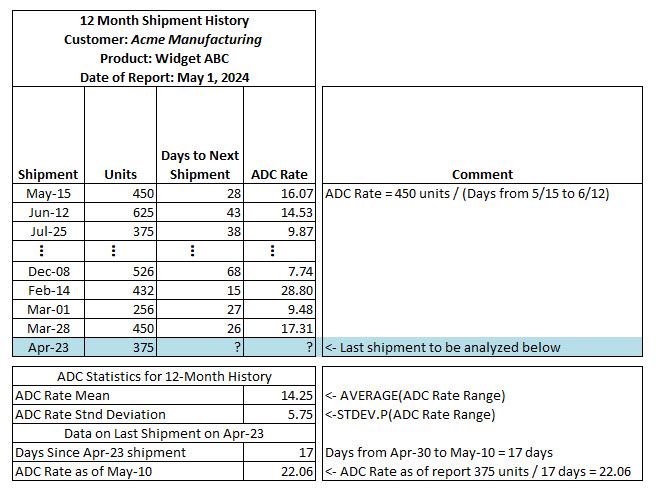
The metric that we are going to analyze is the Average Daily Consumption (ADC) Rate for each product.  We derive our ADC Rate by looking at each shipment over the past 12 months, beginning with the oldest shipment.  Starting with the oldest shipment, we record that date and the number of units shipped.  Looking at Exhibit 2 below, you can see that the oldest shipment was 450 units on May 15th.  Next, we look at the shipment immediately following the first shipment and determine the number of days between those two shipments, which in this case was 28 days (28 days from May 15th, the first shipment date to the second shipment date on June 12th).  We then divide the number of units in the first shipment by the number of days to the second shipment to determine the ADC Rate (16.07 units per day for the first shipment in the series).  Then we do this same process for all the shipments in the 12-month window we are analyzing, except the newest shipment on April 23rd.  The April 23rd shipment is the one that we will be analyzing to compute the probability that the shipment has been depleted by May 10th, May 20th, May 30th and June 9th.

The ADC Rate is determined by dividing the units in the first shipment by the days to the second shipment, resulting in an ADC Rate of 16.07 units per day for the initial shipment. This process is replicated for all shipments within the 12-month analysis window, except for the latest shipment on April 23rd. This April 23rd shipment forms the basis of our analysis to compute the probability of depletion by May 10th, May 20th, May 30th, and June 9th

From the summarized overview below, you can observe details about shipments such as the May 15th shipment (450 units and 16.07 ADC Rate), the June 12th shipment (625 units and 14.53 ADC Rate), and subsequent entries up to the latest shipment on April 23rd, consisting of 375 units. Directly below this summary, the average of the ADC Rates is 14.25 units per day, accompanied by a Standard Deviation of 5.75 units.  These are the values that we will be inputting to the NORM.DIST() function to compute the cumulative probability distributions.

Immediately following on the summary, there is additional information relevant to the initial analysis period starting on May 10th. This includes the Days Since the April 23rd shipment (17 days) and the corresponding ADC Rate effective on May 10th, which stands at 22.06 units.

How NORM.DIST() Function Produces Our Business Analytics

Above we determined the mean ADC Rate for the prior 12 months was 14.25 units per day with a standard deviation of 5.75 units.  As of May 1, 2024, the customer has not requested another shipment of this product since the April 23rd shipment.  As we can see from the monthly calculations above for each shipment, there is a fair amount of variance between each shipment ADC Rate from period to period.  As with most companies, our Sales Reps are very busy, visiting customers.  We want to know with some confidence that the customer has depleted or is about to fully deplete their most recent shipment–the April 23rd shipment in this case.  Exhibit 3 below provides some additional detail to the calculations used to determine the probability of the most recent.  If you look in the last column, we have listed the computed probabilities of that shipment being consumed.  As of May 10th (17 days past the last shipment date), there is only a 9% chance, but it quickly increases to 86% by June 9th (47 days after the last shipment date). 

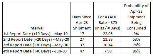
The Probability of Shipment Being Consumed metric above, for all the dates is as follow:

May 10th Date —>  1 – NORM.DIST(22.06,14.25,5.75) = 9%

May 20th Date —>  1 – NORM.DIST(13.89,14.25,5.75) = 53%

May 30th Date —>  1 – NORM.DIST(10.14,14.25,5.75) = 76%

June 9th Date —>  1 – NORM.DIST(7.98,14.25,5.75) = 86%

If you are wondering why we have to subtract by 1.0, you need to understand that the NORM.DIST() function is computing the cumulative probabilities beginning at X = 0 essentially.  What we want, for example in the May 10th Date computation is what is the probability that this customer depleted their last shipment in an ADC Rate of 22.06 or higher.  This graphic may help crystalize what is being computed for the May 10th metric.

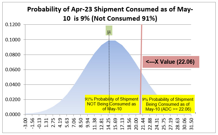
Hopefully this makes it clear that we want the area under the curve to the right of our X value of 22.06, but the NORM.DIST() function gives us the part of the curve to the left of our X value.  Subtracting by 1.00 works because the total area under the curve is 1.00 or 100% probability.

A Usage for the NORM.INV() in Our Application

Through this strategic business analysis discussion, we have been focused on utilizing the NORM.DIST() function; consequently, you may be wondering how NORM.INV() would fit it into our analysis.  Let’s assume that the Sales Operations Team has decided that any product that gets to a 95% probability of being depleted merits a call on that date.  This is very simple, but it requires a couple of steps.  First step is compute what X value gets us to the 95% cumulative probability of depletion, which would be as follows:

X That Equates to 95% Probability of Depletion = NORM.INV((1-.95),14.25,5.75) = 4.792

Here we have to subtract our 95% probability from 1.00 to get a curve percentage of 5%.  The above 5% Target X of 4.792 is the ADC Rate a customer would have to achieve to get to the 95% probability of depleting their last shipment.  We have to now convert the 4.792 ADC into days using the last shipment of 375 Units as follows:

Date That Equals 95% Depletion = April, 23, 2024 + ROUND((375 / 4.792),0) = July 24, 2024 (we had to add 78 days to get a 4.792 depletion rate)

This calculation could be added to the Consumption Analysis Report as an additional data for the Sales Reps.  Clearly this is very computationally intensive and requires custom Visual Basic.  If you have an interest in producing more insightful analysis for your Sales Reps, contact us about getting this customer application modified for your business.  The application is designed to produce all separate reports for each Sales Rep and email the Excel workbook to each Sales Rep and their territory manager.  Contact us today!

Hopefully you found this enlightening and can utilize it in your own organizations.  If you need help setting up standard costs, or inventory reduction processes, please give us call.  We have the tools to help.